【计算机视觉】基于BOW的图像检索（Python）

一、Bow（Bag of words）模型简介

1.1 原理

• Bag of words模型最初被用在文本分类中，将文档表示成特征矢量。它的基本思想是假定对于一个文本，忽略其词序和语法、句法，仅仅将其看做是一些词汇的集合，而文本中的每个词汇都是独立的。
• 简单说就是将每篇文档都看成一个袋子（因为里面装的都是词汇，所以称为词袋，Bag of words即因此而来），然后根据袋子里装的词汇对其进行分类。如文档中猪、马、牛、羊、山谷、土地、拖拉机这样的词汇多些，而银行、大厦、汽车、公园这样的词汇少些，我们就倾向于判断它是一篇描绘乡村的文档，而不是描述城镇的。
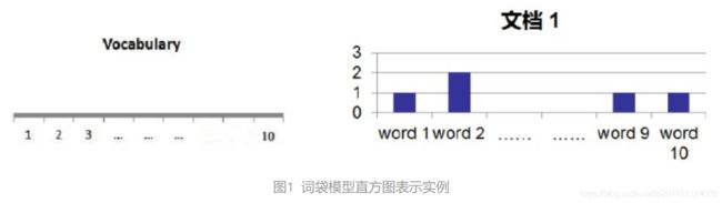
• 根据每个单词在文本中出现的权重，便可构造单词的频率直方图。词表就相当于直方图的基，新来要表述的文档向这个基上映射。
  

1.2 模型应用到图像检索中

为了表示一幅图像，我们可以将图像看作文档，即若干个“视觉词汇”的集合，同样的，视觉词汇之间没有顺序。

1.2.1 特征提取

• 由于图像中的词汇不像文本文档那样是现成的单词，所以我们首先要从图像中提取出相互独立的视觉词汇。然后为创建视觉单词词汇，第一步要做的就是提取特征描述子。
• SIFT算法是提取图像中局部不变特征的应用最广的算法，所以我们可以采用SIFT算法才进行特征提取。
• 将每幅图像提取出的描述子保存在一个文件中，构建视觉词典。

1.2 2 学习 “视觉词典（visual vocabulary）”

聚类是实现 visual vocabulary /codebook的关键 ，最常见的聚类方法就是，K-means 聚类算法。

（1）随机初始化 K 个聚类中心

（2）对应每个特征，根据距离关系赋值给某个中心/类别 。其中距离的计算可采用欧式距离：

（3）对每个类别，根据其对应的特征集重新计算聚类中心
重复（2）、（3）步骤，直至算法收敛

1.2.3 针对输入特征集，根据视觉词典进行量化

对于输入特征，量化的过程是将该特征映射到距离其最接近的视觉单词，并实现计数 。选择合适的视觉词典的规模是我们需要考虑的问题，若规模太少，会出现视觉单词无法覆盖所有可能出现的情况 。若规模太多，又会计算量大，容易过拟合 。只能通过不断的测试，才能找到最合适的词典规模。

1.2.4 把输入图像转化成视觉单词（visual words） 的频率直方图
利用SIFT算法，可以从每幅图像中提取很多特征点，通过统计每个视觉单词在词汇中出现的次数，可以获得直方图。

1.2.5 构造特征到图像的倒排表，通过倒排表快速索引相关图像
用K邻近算法，进行图像的检索。给定输入图像的BOW直方图, 在数据库中查找 k 个最近邻的图像 。对于图像分类问题，可以根据这k个近邻图像的分类标签， 投票获得分类结果 。

1.2.6 根据索引结果进行直方图匹配
我们可以利用建立起来的索引找到包含特定单词的所有图像。为了获得包含多个单词的候选图像，有两种解决方法。
（1）我们可以在每个单词上进行遍历，得到包含该单词的所有图像，然后合并这些列表。接着对在合并了的列表中，对每一个图像id出现的次数进行跟踪排序，排在列表最前面的是最好的匹配图像。
（2）如果不想遍历所有的单词，可以根据其倒排序文档频率权重进行排序，并使用那些权重最高的单词，在这些单词上进行遍历，减少计算量，提高运行的效率。

二、图像检索实验

2.1 特征提取+生成词汇

• 对每张图片生成相应的.sift文件，及视觉词汇，以便建立BOW模型。此处用的是图像集为100张。1000个单词的词汇表，在K-means聚类阶段训练数据，聚成指定的10类。

2.1.1 实现代码

# -*- coding: utf-8 -*-

import pickle

from PCV.imagesearch import vocabulary

from PCV.tools.imtools import get_imlist

import sift

# 获取图像列表

imlist = get_imlist('D:/Python/ComputerView/test1/first1000/')

nbr_images = len(imlist)

# 获取特征列表

featlist = [imlist[i][:-3] + 'sift' for i in range(nbr_images)]

# 提取文件夹下图像的sift特征

for i in range(nbr_images):
    sift.process_image(imlist[i], featlist[i])

# 生成词汇

voc = vocabulary.Vocabulary('ukbenchtest')

voc.train(featlist, 100, 10)

# 保存词汇

# saving vocabulary

with open('D:/Python/ComputerView/test1/first1000/vocabulary.pkl', 'wb') as f:

    pickle.dump(voc, f)

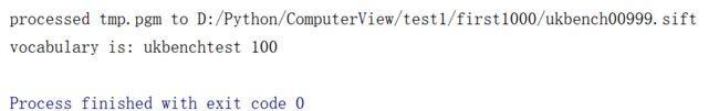
print('vocabulary is:', voc.name, voc.nbr_words)

2.1.2 实现结果

图片sift特征提取：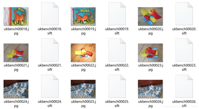
生成的视觉词汇：

2.2 建立图像索引+存放数据模型

• 在开始之前，需要创建表，索引和索引器indexer类，以便将图像数据写入数据库，将上面得到的数据模型存放数据库testImaAdd.db中。

2.2.1 实现代码

# -*- coding: utf-8 -*-

import pickle

from PCV.imagesearch import imagesearch

from PCV.localdescriptors import sift

import sqlite3

from PCV.tools.imtools import get_imlist

# 获取图像列表

imlist = get_imlist('D:/Python/ComputerView/test1/first1000/')

#imlist = get_imlist('E:/Python37_course/test7/images/')

nbr_images = len(imlist)

# 获取特征列表

featlist = [imlist[i][:-3] + 'sift' for i in range(nbr_images)]

# load vocabulary

# 载入词汇

with open('D:/Python/ComputerView/test1/first1000/vocabulary.pkl', 'rb') as f:

    voc = pickle.load(f)

# 创建索引

indx = imagesearch.Indexer('testImaAdd.db', voc)

indx.create_tables()

# go through all images, project features on vocabulary and insert

# 遍历所有的图像，并将它们的特征投影到词汇上


# for i in range(nbr_images)[:1000]:

for i in range(nbr_images)[:100]:
    locs, descr = sift.read_features_from_file(featlist[i])

    indx.add_to_index(imlist[i], descr)

# commit to database

# 提交到数据库

indx.db_commit()

con = sqlite3.connect('testImaAdd.db')

print(con.execute('select count (filename) from imlist').fetchone())

print(con.execute('select * from imlist').fetchone())

2.2.2 实现结果

索引的建立：

成功建立图像数据库：

2.3 图像索引测试

2.3.1 实现代码

# -*- coding: utf-8 -*-

import pickle

import sift

from PCV.imagesearch import imagesearch

from PCV.geometry import homography

from PCV.tools.imtools import get_imlist

# load image list and vocabulary

# 载入图像列表

imlist = get_imlist('D:/Python/ComputerView/test1/first1000/')

nbr_images = len(imlist)

# 载入特征列表

featlist = [imlist[i][:-3 ] +'sift' for i in range(nbr_images)]

# 载入词汇

with open('D:/Python/ComputerView/test1/first1000/vocabulary.pkl', 'rb') as f:

    voc = pickle.load(f)

src = imagesearch.Searcher('testImaAdd.db' ,voc)

# index of query image and number of results to return

# 查询图像索引和查询返回的图像数

q_ind = 0

nbr_results = 20

# regular query

# 常规查询(按欧式距离对结果排序)

res_reg = [w[1] for w in src.query(imlist[q_ind])[:nbr_results]]

print('top matches (regular):', res_reg)

# load image features for query image

# 载入查询图像特征

q_locs ,q_descr = sift.read_features_from_file(featlist[q_ind])

fp = homography.make_homog(q_locs[:, :2].T)



# RANSAC model for homography fitting

# 用单应性进行拟合建立RANSAC模型

model = homography.RansacModel()

rank = {}



# load image features for result

# 载入候选图像的特征

for ndx in res_reg[1:]:

    locs ,descr = sift.read_features_from_file(featlist[ndx])  # because 'ndx' is a rowid of the DB that starts at 1

    # get matches

    matches = sift.match(q_descr ,descr)

    ind = matches.nonzero()[0]

    ind2 = matches[ind]

    tp = homography.make_homog(locs[: ,:2].T)

    # compute homography, count inliers. if not enough matches return empty list

    try:

        H ,inliers = homography.H_from_ransac(fp[: ,ind] ,tp[: ,ind2] ,model ,match_theshold=4)

    except:

        inliers = []

    # store inlier count

    rank[ndx] = len(inliers)



# sort dictionary to get the most inliers first

sorted_rank = sorted(rank.items(), key=lambda t: t[1], reverse=True)

res_geom = [res_reg[0] ] +[s[0] for s in sorted_rank]

print ('top matches (homography):', res_geom)



# 显示查询结果

imagesearch.plot_results(src ,res_reg[:11])  # 常规查询

imagesearch.plot_results(src ,res_geom[:11])  # 重排后的结果

2.3.2 实现结果

待索引图像：

常规查询结果：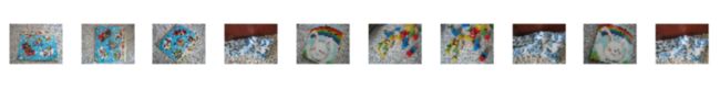
重排后的查询结果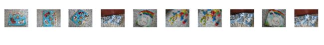：对于常规查询结果和重排后的查询结果来说，重排后的查询结果会比常规查询结果更为准确些，重排用单应性进行拟合建立RANSAC模型，再导入候选图像特征进行排序查询；常规查询只是进行了简单的索引和查询，找到相似即可。

三、实验小结

3.1 问题及解决

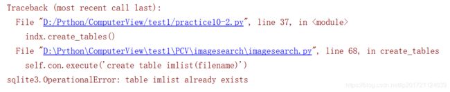
出现上面情况，说明已经生成一个数据库，如果需要再生成一个需要，把之前的数据库文件删除，或者重新生成另外一个库即换一个库名。建议直接删除。删除后，运行结果就会在项目下生成一个DB文件。

3.2 实验收获

基于BOW的图像检索有一定的优势，检测出的结果相对理想，但其不足之处也显而易见：

1、使用k-means聚类，除了其K和初始聚类中心选择的问题外，对于海量数据，输入矩阵的巨大将使得内存溢出及效率低下。Kmeans聚类时间长，速度慢；

2、词袋表征特征的过程其实牵涉到量化的过程，这其实损失了特征的精度，使精度低下；

3、字典大小的选择不好控制，字典过大，单词缺乏一般性，对噪声敏感，计算量大，关键是图象投影后的维数高；字典太小，单词区分性能差，对相似的目标特征无法表示；

4、将图像表示成一个无序局部特征集的特征包方法，丢掉了所有的关于空间特征布局的信息，在描述性上具有一定的有限性。