倍分法DID详解 (二):多时点 DID (渐进DID)
2020寒假Stata现场班
北京, 1月8-17日,连玉君-江艇主讲

2020连享会-文本分析与爬虫-现场班
西安, 3月26-29日,司继春-游万海 主讲; (附助教招聘)

作者:王昆仑 (天津大学)
Stata连享会 计量专题 || 公众号合集

导入
在 「连享会 - 倍分法系列推文」—— 「倍分法DID详解 (一):传统 DID」 文中,我们详细介绍了 DID 模型的估计,平行趋势的检验以及政策的动态效果的展示等主题,并通过模拟的方式给出了较为详尽的解答。
但该文中仅仅针对实施时点为统一的年份将样本划分为实验组和控制组的 Standard DID 模型。本文作为本系列的第二篇文章,将对政策实施时点更加灵活的 DID 形式进行介绍,其主要内容结构和方法与上一篇尽量保持一致,以达到本系列开篇时所说的用一套模拟方法将 Standard DID 和 Time-varying DID 模型整合在一起的目的。
一、引言
标准 DID 模型一般针对政策实施时点为同一个时期,且接受干预的状态将一直持续下去,否则 T r e a t i ∗ P o s t t Treat _i * Post _t Treati∗Postt 的交互项设置将会严重违背平行趋势的假设,从而导致交互项的估计系数有偏。由于现实世界中很多的政策试点地区和时间都不尽相同,而且也容易发生个体是否接受政策干预的状态在不停地发生改变,因此,本文将介绍渐进 DID 方法(Time-varying DID)来使得 DID 模型更加具有一般性。这类模型也被称为多时点 DID。 陈强老师在推文中称为“异时 DID (heterogeneous timing DID)”。
高铁开通、官员晋升以及多阶段试点政策等主题往往应用渐进 DID 方法作为其主要方法。说到渐进 DID 的相关论文,不得不提到的就是发表在 The Journal of Finance 上的 Beck, Levine & Levkov(2010) 这篇文章。 它运用渐进 DID 方法对银行去管制对收入分配的影响,并且给出渐进 DID 模型的平行趋势检验的方法。这篇不失为一篇利用渐进 DID 的模版。关于 Beck, Levine & Levkov(2010)更多的讨论,请参见经管之家黄河泉老师的帖子,这篇文章的代码和数据也可以从这个帖子中下载得到。我们在本文的第五节对 Beck, Levine & Levkov(2010) 的 Figure 3 进行复现。
下面对Standard DID 和 Time-varying DID 的模型设定予以简要的介绍。在双重固定效应(Two-Way Fixed Effects)的估计框架下,Standard DID 的一般化方程是 Y i t = β 0 + β 1 ∗ T r e a t i ∗ P o s t t + β ∗ Σ Z i t + μ i + τ t + ϵ i t ( 1 ) Y_{it} = \beta_0 + \beta_1 * Treat_i * Post_t + \beta * \Sigma Z_{it} + \mu_i + \tau_t + \epsilon_{it} \quad (1) Yit=β0+β1∗Treati∗Postt+β∗ΣZit+μi+τt+ϵit(1)
与之相对应的Time-varying DID 的一般化模型设定是 Y i t = β 0 + β 1 ∗ T r e a t i t + β ∗ Σ Z i t + μ i + τ t + ϵ i t ( 2 ) Y_{it} = \beta_0 + \beta_1 * Treat_{it} + \beta * \Sigma Z_{it} + \mu_i + \tau_t + \epsilon_{it} \quad (2) Yit=β0+β1∗Treatit+β∗ΣZit+μi+τt+ϵit(2)
其中, Σ Z i t \Sigma Z_{it} ΣZit 表示随时间和个体变化的控制变量, μ i \mu_i μi 表示个体固定效应, τ t \tau_t τt 表示时间固定效应, ϵ i t \epsilon_{it} ϵit 表示标准残差项,$ i = 1,2,3,…,N; t = 1,2,3,…,T$ 。公式(1)和公式(2)中最重要的区别就是 T r e a t i ∗ P o s t t Treat_i * Post_t Treati∗Postt和 T r e a t i t Treat_{it} Treatit 。换句话说,Time-varying DID 用一个随时间和个体变化的处理变量代替 Standard DID 中常用的交互项。
二、Time-varyig DID Simulation: 政策效果不随时间发生变化
2.1 模拟数据的生成
再次仿照 「倍分法DID详解 (一):传统 DID」 文中生成基础的数据结构,依然为60个体*10年=600个观察值的平衡面板数据。Time-varying DID 的设置体现在,我们使得 id 编号为 1-20 的个体在 2004 年接收政策干预,编号 21-40 的个体在 2006 年接受干预,编号为 41-60 的个体在 2008 年接受干预。因此,三组个体接受政策干预的时长分别为 6 年,4 年和 2年。
///设定60个观测值,设定随机数种子
. clear all
. set obs 60
. set seed 10101
. gen id =_n

/// 每一个数值的数量扩大11倍,再减去前六十个观测值,即60*11-60 = 600,为60个体10年的面板数据
. expand 11
. drop in 1/60
. count

///以id分组生成时间标识
. bys id: gen time = _n+1999
. xtset id time

///生成协变量以及个体和时间效应
. gen x1 = rnormal(1,7)
. gen x2 = rnormal(2,5)

. sort time id
. by time: gen ind = _n
. sort id time

. by id: gen T = _n
. gen y = 0

///生成处理变量,此时D为Dit,设定1-20在2004年接受冲击,21-40为2006年,36-60为2008年
. gen D = 0
. gen birth_date = 0

forvalues i = 1/20{
	replace D = 1 if id  == `i' & time >= 2004
	replace birth_date = 2004 if id == `i'
}

forvalues i = 21/40{
	replace D = 1 if id  == `i' & time >= 2006
	replace birth_date = 2006 if id == `i'
}

forvalues i = 41/60{
	replace D = 1 if id  == `i' & time >= 2008
	replace birth_date = 2008 if id == `i'
}

///将基础数据结构保存成dta文件,命名为DID_Basic_Simu.dta,默认保存在当前的 working directory 路径下

save "DID_Basic_Simu_1.dta", replace
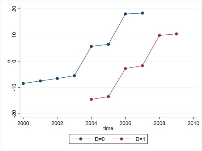
生成结果变量,设定接受干预个体的政策效果为 10。利用固定效应模型消除个体效应和 x1、x2 两个变量对结果变量的影响,得到残差,画出更加干净分组的结果变量的时间趋势图。这个图形可以作为验证平行趋势的一个旁证。
///调用生成的基础数据文件
clear
use "DID_Basic_Simu_1.dta"

///Y的生成,使得接受冲击的个体的政策真实效果为10
bysort id: gen y0 = 10  + 5 * x1 + 3 * x2 + T + ind  + rnormal()
bysort id: gen y1 = 10  + 5 * x1 + 3 * x2 + T + ind  + 10 + rnormal() if time >= 2004 & id >= 1 & id <= 20
bysort id: replace y1 = 10  + 5 * x1 + 3 * x2 + T + ind  + 10 + rnormal() if time >= 2006 & id >= 21 & id <= 40
bysort id: replace y1 = 10  + 5 * x1 + 3 * x2 + T + ind  + 10 + rnormal() if time >= 2008 & id >= 41 & id <= 60
bysort id: replace y1 = 10  + 5 * x1 + 3 * x2 + T + ind  + rnormal() if y1 == .

replace y = y0 + D * (y1 - y0)

///去除个体效应和协变量对Y的影响,得到残差并画图
xtreg y x1 x2 , fe r
predict e, ue
binscatter e time, line(connect) by(D)

///输出生成的图片,令格式为800*600
graph export "article2_1.png",as(png) replace width(800) height(600)
2.2 多种估计结果的呈现
继续使用双向固定效应(Two-Way Fixed Effects)的方法设定方程,使用 reg, xtreg, areg, reghdfe 等四个 Stata 命令进行估计,四个命令的比较放在了下方的表格中。在本文中,主要展示命令’reghdfe’的输出结果,该命令的具体介绍可以参考 Stata: reghdfe-多维固定效应。
| reg | xtreg | areg | reghdfe | |
|---|---|---|---|---|
| 个体固定效应 | i.id | xtreg,fe | areg,absorb(id) | absorb(id time) |
| 时间固定效应 | i.time | i.time | i.time | absorb(id time) |
| 估计方法 | OLS | 组内去平均后OLS | OLS | OLS |
| 优点 | 命令熟悉,逻辑清晰 | 固定效应模型的官方命令 | 官方命令,可以提高组别不随样本规模增加的估计效率 | 高维固定效应模型,可以极大提到估计效率,且选项多样,如支持多维聚类 |
| 缺点 | 运行速度慢,结果呈现过多不太需要的固定效应的结果 | 需要手动添加时间固定效应 | 需要手动添加时间固定效应 | 无 |
. reghdfe y c.D x1 x2, absorb(id time) vce(robust)
+-----------------------------------------------------------------------------+
(converged in 3 iterations)

HDFE Linear regression                            Number of obs   =	       600
Absorbing 2 HDFE groups                           F(   3,    528) =  282958.86
Statistics robust to heteroskedasticity           Prob > F        =	    0.0000
                                                  R-squared       =	    0.9996
                                                  Adj R-squared   =	    0.9995
                                                  Within R-sq.    =	    0.9994
                                                  Root MSE        =	    0.9630
+-----------------------------------------------------------------------------+
     |               Robust
    y|      Coef.   Std. Err.      t     P>t     [95% Conf.	Interval]
+-----------------------------------------------------------------------------+
    D|   9.884974   .1571734    62.89   0.000     9.576212	10.19374
   x1|   4.995274   .0056514   883.90   0.000     4.984172	5.006376
   x2|   2.998722   .0083092   360.89   0.000     2.982399	3.015045
+-----------------------------------------------------------------------------+

Absorbed degrees of freedom:
+--------------------------------------------------------+
Absorbed FE|  Num. Coefs.  =   Categories  -   Redundant
+--------------------------------------------------------+
        id |          60              60              0
      time |           9              10              1
+--------------------------------------------------------+
///保存并输出多个命令的结果
reg y c.D x1 x2 i.time i.id, r
eststo reg
xtreg y c.D x1 x2 i.time, r fe
eststo xtreg_fe
areg y c.D x1 x2 i.time, absorb(id) robust
eststo areg
reghdfe y c.D x1 x2, absorb(id time) vce(robust)
eststo reghdfe

estout *, title("The Comparison of Actual Parameter Values") ///
		 cells(b(star fmt(%9.3f)) se(par)) ///
		 stats(N N_g, fmt(%9.0f %9.0g) label(N Groups)) ///
		 legend collabels(none) varlabels(_cons Constant) keep(x1 x2 D)

+--------------------------------------------------------------------------------+
                            The Comparison of Actual Parameter Values
+--------------------------------------------------------------------------------+
       |              reg           xtreg_fe	     areg	    reghdfe
+--------------------------------------------------------------------------------
     D |            9.885***        9.885***	    9.885***	9.885***
       |            (0.157)         (0.139)	        (0.157)     (0.157)
    x1 |            4.995***        4.995***	    4.995***	4.995***
       |            (0.006)         (0.006)	        (0.006)	    (0.006)
    x2 |            2.999***        2.999***	    2.999***	2.999***
       |            (0.008)         (0.009)	        (0.008)	    (0.008)
+--------------------------------------------------------------------------------+
N      |              600             600	            600	        600
Groups |                               60
+--------------------------------------------------------------------------------+
* p<0.05, ** p<0.01, *** p<0.001
+--------------------------------------------------------------------------------+
四组回归结果中交互项和协变量的估计系数和标准误几乎完全相同(唯一的区别在于 xtreg_fe 估计项系数的标准差),并且都十分接近于模拟生成时的设定值,说明方程设定和使用的估计方法是合适的。 D i t D_{it} Dit 的四个估计系数都为9.885,其95%CI明显包含真实效果 10, 因此方程的设定不存在问题。从表格展示的结果可以知道,四个命令估计的系数大小是一致的,唯一的区别在于固定效应模型的估计系数其标准误略有变化。再次验证了这四个命令在估计Two-Way Fixed Effects 上是等价的。
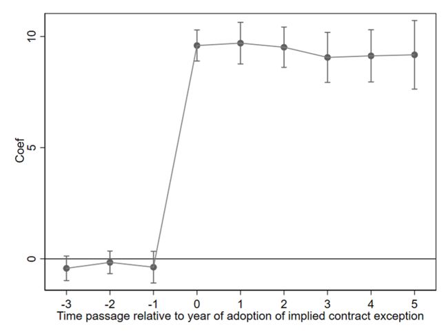
2.3 ESA 方法应用 (Event Study Approach)
本部分对 DID 模型和事件研究法 (Event Study Approach) 的结合做出介绍。 DID 应用 ESA 方法有两个目的:一是可以利用回归方法对双重差分法中最重要的平行趋势假设进行检验,与上面的图示法相比,好处在于可以控制协变量的影响,方程形式也更加灵活;二是可以更加清楚地得到政策效果在时间维度上地变化。因此,这部分检验在论文中也往往被称为政策的动态效果(Dynamic Effects) 或者灵活的 DID (Flexible DID Estimates)。
因此,对于 Standard DID 方法来说,由于具有相同的政策干预时点,因此只需要产生政策虚拟变量和每个时期的虚拟变量的交互项,然后选择其中一个交互项作为对照组,将因变量回归到剩下的交互项上,观察每一个交互项的系数即可得到政策所产生的动态效果。在具体的实践中,所选择的作为对照组的交互项,往往是初期、政策前一期和政策当期,详细操作见本系列第一篇推文 「倍分法DID详解 (一):传统 DID」 第五节。
然而,由于该方法对于所有个体没有一个统一的政策时点,且进入实验组的个体在不断变化,因此上述的流程无法应用到 Time-varying DID 方法上。这时候我们需要换一个角度思考生成时期虚拟变量的这个问题:在 Standard DID 设置中,由于进入实验组的个体和时间都是固定的,因此政策和时期二者虚拟变量的生成还隐含着另一层意思,即对于每一个个体来说,生成固定的时期虚拟变量就顺理成章地有了政策的前一期,前二期,…,到前 N 期,和后一期,后二期,…到后 N 期。因此,对于 Time-varying DID 来说,即使没有了统一的政策时点,由于每一个个体进入实验组的时点是确定的,我们可以通过当前年份与该个体的政策时点相比较,就可以得到该个体的前 N 期到后 N 期,从而观察动态的政策效果。换句话说,Standard DID 结合 ESA 方法所生成的时期虚拟变量是一种绝对的时间尺度,即观测政策在某个样本时期的效果,而 Time-varying DID 利用 ESA 方法所需要的是相对的时期,即观测政策效果在个体接受处理的前 N 期和后 N 期的变化。
///调用生成的基础数据文件
clear
use "DID_Basic_Simu_1.dta"

///Y的生成,使得接受冲击的个体的政策真实效果为10
bysort id: gen y0 = 10  + 5 * x1 + 3 * x2 + T + ind  + rnormal()
bysort id: gen y1 = 10  + 5 * x1 + 3 * x2 + T + ind  + 10 + rnormal() if time >= 2004 & id >= 1 & id <= 20
bysort id: replace y1 = 10  + 5 * x1 + 3 * x2 + T + ind  + 10 + rnormal() if time >= 2006 & id >= 21 & id <= 40
bysort id: replace y1 = 10  + 5 * x1 + 3 * x2 + T + ind  + 10 + rnormal() if time >= 2008 & id >= 41 & id <= 60
bysort id: replace y1 = 10  + 5 * x1 + 3 * x2 + T + ind  + rnormal() if y1 == .
replace y = y0 + D * (y1 - y0)

///Time-varying DID 和 Event Study Approach 的结合

///用当前年份减去个体接受处理的年份,得到相对的时间值event,将 -4 期之前的时间归并到第 -4 期,由于部分个体没有多于 -4 期的时间
///然后生成相对时间值的虚拟变量,eventt,并将首期设定为基准对照组
gen event = time - birth_date
replace event = -4 if event <= -4
tab event, gen(eventt)
drop eventt1

xtreg y eventt* x1 x2 i.time, r fe

coefplot, ///
   keep(eventt*)  ///
   coeflabels(eventt2 = "-3"   ///
   eventt3 = "-2"             ///
   eventt4 = "-1"             ///
   eventt5 = "0"              ///
   eventt6  = "1"             ///
   eventt7  = "2"             ///
   eventt8  = "3"             ///
   eventt9  = "4"             ///
   eventt10 = "5")           ///
   vertical                       ///
   yline(0)                       ///
   ytitle("Coef")               ///
   xtitle("Time passage relative to year of adoption of implied contract exception") ///
   addplot(line @b @at)                 ///
   ciopts(recast(rcap))                 ///
   scheme(s1mono)

///输出生成的图片,令格式为800*600
graph export "article2_2.png",as(png) replace width(800) height(600)
连享会计量方法专题……
三、Time-varyig DID Simulation: 政策效果随时间发生变化
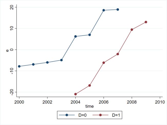
3.1 模拟数据的生成
调用在本文第二节生成并保存的的基础数据文件“DID_Basic_Simu_1.dta"”。依然设定 id 编号为 1-20 的个体在 2004 年接收政策干预,编号 21-40 的个体在 2006 年接受干预,编号为 41-60 的个体在 2008 年接受干预。因此,三组个体接受政策干预的时长分别为 6 年,4 年和 2年。
结果变量的生成与 2.1 节略有变化,我们将真实的政策效果设定为在政策发生当期个体的结果变量增加三个单位,以后每多一期,再增加三个单位。
然后利用固定效应模型去除个体效应和协变量 x1,x2 的影响,画出更加干净的结果变量的图像,作为验证平行趋势的旁证。
///调用生成的基础数据文件
clear
use "DID_Basic_Simu_1.dta"

///Y的生成,设定真实的政策效果为当年为3,并且每年增加3
bysort id: gen y0 = 10  + 5 * x1 + 3 * x2 + T + ind + rnormal()
bysort id: gen y1 = 10  + 5 * x1 + 3 * x2 + T + ind  + (time - birth + 1 ) * 3 + rnormal() if time >= 2004 & id >= 1 & id <= 20
bysort id: replace y1 = 10  + 5 * x1 + 3 * x2 +  T + ind  + (time - birth + 1 ) * 3  + rnormal() if time >= 2006 & id >= 21 & id <= 40
bysort id: replace y1 = 10  + 5 * x1 + 3 * x2 +  T + ind  + (time - birth + 1 ) * 3  + rnormal() if time >= 2008 & id >= 41 & id <= 60
bysort id: replace y1 = 10  + 5 * x1 + 3 * x2 +  T + ind  + rnormal() if y1 == .

replace y = y0 + D * (y1 - y0)

///去除个体效应和协变量对Y的影响,得到残差并画图
xtreg y x1 x2 , fe r
predict e, ue
binscatter e time, line(connect) by(D)

///输出生成的图片,令格式为800*600
graph export "article2_3.png",as(png) replace width(800) height(600)
3.2 多种估计结果的呈现
依然使用双向固定效应(Two-Way Fixed Effects)的方法设定方程,使用reg,xtreg,areg,reghdfe等四个Stata命令进行估计。在本文中,主要展示命令’reghdfe’的输出结果,该命令的具体介绍可以参考 Stata: reghdfe-多维固定效应。
. reghdfe y c.D x1 x2, absorb(id time) vce(robust)
+-----------------------------------------------------------------------------+
(converged in 3 iterations)

HDFE Linear regression                            Number of obs   =	     600
Absorbing 2 HDFE groups                           F(   3,    528) =	49885.71
Statistics robust to heteroskedasticity           Prob > F        =	  0.0000
                                                  R-squared       =	  0.9973
                                                  Adj R-squared   =	  0.9970
                                                  Within R-sq.    =	  0.9964
                                                  Root MSE        =	  2.3386

+-----------------------------------------------------------------------------+
      |              Robust
    y |     Coef.   Std. Err.      t         P>t       [95% Conf. Interval]
+-----------------------------------------------------------------------------+
    D |    2.69066   .3612682     7.45       0.000     1.980961	3.40036
    x1|   4.987876   .0138214   360.88       0.000     4.960725	5.015028
    x2|   3.026438   .0201725   150.03       0.000      2.98681	3.066066
+-----------------------------------------------------------------------------+

Absorbed degrees of freedom:
+--------------------------------------------------------+
Absorbed FE|  Num. Coefs.  =   Categories  -   Redundant
+--------------------------------------------------------+
        id |          60              60              0
      time |           9              10              1
+--------------------------------------------------------+
///保存并输出多个命令的结果
reg y c.D x1 x2 i.time i.id, r
eststo reg
xtreg y c.D x1 x2 i.time, r fe
eststo xtreg_fe
areg y c.D x1 x2 i.time, absorb(id) robust
eststo areg
reghdfe y c.D x1 x2, absorb(id time) vce(robust)
eststo reghdfe

estout *, title("The Comparison of Actual Parameter Values") ///
		 cells(b(star fmt(%9.3f)) se(par)) ///
		 stats(N N_g, fmt(%9.0f %9.0g) label(N Groups)) ///
		 legend collabels(none) varlabels(_cons Constant) keep(x1 x2 D)


+--------------------------------------------------------------------------------+
The Comparison of Actual Parameter Values
+--------------------------------------------------------------------------------+
          |             reg        xtreg_fe	        areg	    reghdfe
+--------------------------------------------------------------------------------+
        D |         2.691***        2.691***	    2.691***	2.691***
          |         (0.361)         (0.180)	        (0.361)	    (0.361)
        x1|         4.988***        4.988***	    4.988***	4.988***
          |         (0.014)         (0.013)	        (0.014)	    (0.014)
        x2|         3.026***        3.026***	    3.026***	3.026***
          |         (0.020)         (0.020)	        (0.020)	    (0.020)
+--------------------------------------------------------------------------------+
N         |           600             600	            600	    600
Groups    |                            60
+--------------------------------------------------------------------------------+
* p<0.05, ** p<0.01, *** p<0.001
+--------------------------------------------------------------------------------+
四组回归结果中交互项和协变量的估计系数和标准误几乎完全相同(唯一的区别在于 xtreg_fe 估计项系数的标准差),并且都十分接近于模拟生成时的设定值,说明方程设定和使用的估计方法是合适的。 D i t D_{it} Dit的四个估计系数都为2.691,每年的平均处理效应见 3.3 节的图形。从表格展示的结果可以知道,四个命令估计的系数大小是一致的,唯一的区别在于固定效应模型的估计系数其标准误略有变化。再次验证了这四个命令在估计 Two-Way Fixed Effects 上是等价的。
3.3 ESA方法的应用
这部分逻辑与 2.3 节 相同。
///调用生成的基础数据文件
clear
use "DID_Basic_Simu_1.dta"

///Y 的生成,设定真实的政策效果为当年为3,并且每年增加3
bysort id: gen y0 = 10  + 5 * x1 + 3 * x2 + T + ind + rnormal()
bysort id: gen y1 = 10  + 5 * x1 + 3 * x2 + T + ind  + (time - birth + 1 ) * 3 + rnormal() if time >= 2004 & id >= 1 & id <= 20
bysort id: replace y1 = 10  + 5 * x1 + 3 * x2 +  T + ind  + (time - birth + 1 ) * 3  + rnormal() if time >= 2006 & id >= 21 & id <= 40
bysort id: replace y1 = 10  + 5 * x1 + 3 * x2 +  T + ind  + (time - birth + 1 ) * 3  + rnormal() if time >= 2008 & id >= 41 & id <= 60
bysort id: replace y1 = 10  + 5 * x1 + 3 * x2 +  T + ind  + rnormal() if y1 == .

replace y = y0 + D * (y1 - y0)

///Time-varying DID 和 Event Study Approach 的结合
///用当前年份减去个体接受处理的年份,得到相对的时间值 event,将 -4 期之前的时间归并到第 -4 期,由于部分个体没有多于 -4 期的时间
///然后生成相对时间值的虚拟变量,eventt,并将首期设定为基准对照组

gen event = time - birth_date
replace event = -4 if event <= -4
tab event, gen(eventt)
drop eventt1

xtreg y eventt* x1 x2 i.time, r fe

coefplot, ///
   keep(eventt*)  ///
   coeflabels(eventt2 = "-3"   ///
   eventt3 = "-2"           ///
   eventt4 = "-1"           ///
   eventt5 = "0"           ///
   eventt6  = "1"             ///
   eventt7  = "2"              ///
   eventt8  = "3"              ///
   eventt9  = "4"              ///
   eventt10 = "5")            ///
   vertical                             ///
   yline(0)                             ///
   ytitle("Coef")                 ///
   xtitle("Time passage relative to year of adoption of implied contract exception") ///
   addplot(line @b @at)                 ///
   ciopts(recast(rcap))                 ///
   scheme(s1mono)

///输出生成的图片,令格式为800*600
graph export "article2_4.png",as(png) replace width(800) height(600)

连享会计量方法专题……
四、Beck & Levkov(2010) Figure 3 的重现
原图如下:
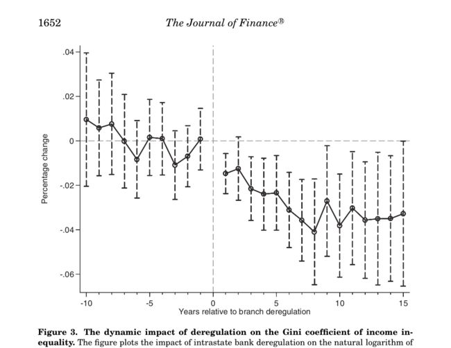
Beck, Levine & Levkov(2010) 原文中所给的绘制 Figure 3 的代码有点繁琐,经过调整和合并,形成本文下面代码。其优点在于,一方面利用 coefplot命令省略大量需要从回归方程中手动提取的系数和%95置信区间端点的取值;另一方面使用循环和 Factor Variables 尽量减少需要生成的过程的变量。对比本节的两张图可知,这部分代码几乎完整地将 Beck, Levine & Levkov(2010)的 Figure 3 重现,并且这部分代码具有普适和易于改造的性质。
提醒:本文并没有提供 Beck, Levine & Levkov(2010) 原文的代码和数据集,本部分的运行结果仅做生成图形对比。感兴趣的同学可以去引言中提到的经管之家黄河泉老师的帖子下载相关内容进行操作。
xtset statefip wrkyr
gen bb = 0
gen aa = 11
gen event = wrkyr - branch_reform

replace event  = -10 if event <= -10
replace event = 15 if event >= 15

///tab event, gen(eventt)
gen event1 = event + 10
gen y = log(gini)

qui xtreg y ib10.event1 i.wrkyr, fe r

///生成前十期系数均值x
forvalues i = 0/9{
	gen b_`i' = _b[`i'.event1]

}

gen avg_coef = (b_0+b_9+b_8+b_7+b_6+b_5+b_4+b_3+b_2+b_1)/10
su avg_coef
return list

coefplot, baselevels ///
   drop(_cons event1  *.wrkyr ) ///
   if(@at!=11) ///去除当年的系数点
   coeflabels(0.event1 = "-10"   ///
   1.event1 = "-9"           ///
   2.event1 = "-8"           ///
   3.event1 = "-7"           ///
   4.event1  = "-6"             ///
   5.event1  = "-5"              ///
   6.event1  = "-4"              ///
   7.event1  = "-3"       ///
   8.event1  = "-2" ///
   9.event1  = "-1" ///
   10.event1 = "0" ///
   11.event1  = "1" ///
   12.event1 = "2" ///
   13.event1  = "3" ///
   14.event1  = "4" ///
   15.event1  = "5" ///
   16.event1  = "6" ///
   17.event1  = "7" ///
   18.event1  = "8" ///
   19.event1 = "9" ///
   20.event1  = "10" ///
   21.event1  = "11" ///
   22.event1 = "12" ///
   23.event1  = "13" ///
   24.event1 = "14" ///
   25.event1 = "15")  ///更改系数的label
   vertical                             ///转置图形
   yline(0, lwidth(vthin) lpattern(dash) lcolor(teal)) ///加入y=0这条虚线
   ylabel(-0.06(0.02)0.06) ///
   xline(11, lwidth(vthin) lpattern(dash) lcolor(teal)) ///
   ytitle("Percentage Changes", size(small)) ///加入Y轴标题,大小small
   xtitle("Years relative to branch deregulation", size(small)) ///加入X轴标题,大小small
   transform(*=@-r(mean)) ///去除前十期的系数均值,更好看
   addplot(line @b @at  if @at < 11, lcolor(gs0)  || line @b @at if @at>11, lcolor(gs0) lwidth(thin))   ///增加点之间的连线
   ciopts(lpattern(dash) recast(rcap) msize(medium))  ///CI为虚线上下封口
   msymbol(circle_hollow) ///plot空心格式
   scheme(s1mono)

///输出生成的图片,令格式为800*600
graph export "article2_6.png",as(png) replace width(800) height(600)

五、总结和拓展
本文承接本系列的第一篇文章,通过数据模拟对 Time-varying DID 方法多种形式的估计,对 Time-varying DID 方法难以直观上理解的平行趋势检验做了分析和展示,依然结合 ESA 方法图示化了政策效果的动态性。如果说需要记住 2.3 节分析中的哪一句话,那就应该是“Standard DID 结合 ESA 方法所生成的时期虚拟变量是一种绝对的时间尺度,而 Time-varying DID 利用 ESA 方法所需要的是相对的时期”。
一般来说,我们认为 DID 方法的识别假设为结果变量的差分形式独立于政策干预,即在差分意义上满足随机实验的要求。因此,从分组的角度来说,DID 方法可以理解为差分意义上的匹配方法,因此在平行趋势检验的时候需要注意结果变量水平值的形式,比如取不取Log,可能会导致平行趋势检验结果的大不同。DID 方法和 ESA 方法的结合利用回归形式检验平行趋势的方法,可以从另一个角度理解其识别假设或者说平行趋势假设:实验组和控制组的固有差异在样本期间的每一个时期内没有发生结构性的变化,政策干预也不会影响到组间固有差异。从 ESA 方法角度去理解即,若原来水平值满足平行趋势假设,那么结果变量差分值就满足 ESA 方法所得到时间窗口期前的估计系数应该都不显著异于零。当然,即使利用一定的方法验证了结果变量具有平行趋势,比如在政策实施前实验组和控制组的变化趋势相同或者 ESA 方法的回归系数接近 0 ,依然无法保证政策实施后的平行趋势依然满足,因为本质上平行趋势假设依然是不可检测的。
细心的同学可能已经发现了,本文中所有个体最终都进入了实验组接受了干预。如果样本中所有个体在样本期末没有完全进入处理组,那么此时,Time-varying DID 的模型设定与本文介绍的过程是否存在什么差别呢,这个问题留在后续的文章中加以解决。
参考资料
- Beck, T., Levine, R., & Levkov, A. (2010). Big bad banks? The winners and losers from bank deregulation in the United States. The Journal of Finance, 65(5), 1637-1667.
- 黄河泉老师的帖子
- 多期DID:平行趋势检验图示
- 开学礼包:如何使用双重差分法的交叉项(迄今最全攻略)
- Stata: reghdfe-多维固定效应
连享会计量方法专题……
附:文中使用的 Stata 代码
情形1: 政策效果不随时间发生变化
. clear all
. set obs 60
. set seed 10101
. gen id =_n

/// 每一个数值的数量扩大11倍,再减去前六十个观测值,即60*11-60 = 600,为60个体10年的面板数据
. expand 11
. drop in 1/60
. count

///以id分组生成时间标识
. bys id: gen time = _n+1999
. xtset id time

///生成协变量以及个体和时间效应
. gen x1 = rnormal(1,7)
. gen x2 = rnormal(2,5)

. sort time id
. by time: gen ind = _n
. sort id time

. by id: gen T = _n
. gen y = 0

///生成处理变量,此时D为Dit,设定1-20在2004年接受冲击,21-40为2006年,36-60为2008年
. gen D = 0
. gen birth_date = 0

forvalues i = 1/20{
	replace D = 1 if id  == `i' & time >= 2004
	replace birth_date = 2004 if id == `i'
}

forvalues i = 21/40{
	replace D = 1 if id  == `i' & time >= 2006
	replace birth_date = 2006 if id == `i'
}

forvalues i = 41/60{
	replace D = 1 if id  == `i' & time >= 2008
	replace birth_date = 2008 if id == `i'
}

///将基础数据结构保存成dta文件,命名为DID_Basic_Simu.dta,默认保存在当前的 working directory 路径下

save "DID_Basic_Simu_1.dta",replace

///调用生成的基础数据文件
clear
use "DID_Basic_Simu_1.dta"

///Y的生成,使得接受冲击的个体的政策真实效果为10
bysort id: gen y0 = 10  + 5 * x1 + 3 * x2 + T + ind  + rnormal()
bysort id: gen y1 = 10  + 5 * x1 + 3 * x2 + T + ind  + 10 + rnormal() if time >= 2004 & id >= 1 & id <= 20
bysort id: replace y1 = 10  + 5 * x1 + 3 * x2 + T + ind  + 10 + rnormal() if time >= 2006 & id >= 21 & id <= 40
bysort id: replace y1 = 10  + 5 * x1 + 3 * x2 + T + ind  + 10 + rnormal() if time >= 2008 & id >= 41 & id <= 60
bysort id: replace y1 = 10  + 5 * x1 + 3 * x2 + T + ind  + rnormal() if y1 == .

replace y = y0 + D * (y1 - y0)

///去除个体效应和协变量对Y的影响,得到残差并画图
xtreg y x1 x2 , fe r
predict e, ue
binscatter e time, line(connect) by(D)

///输出生成的图片,令格式为800*600
graph export "article2_1.png",as(png) replace width(800) height(600)

///保存并输出多个命令的结果
///输出生成的图片,令格式为800*600

reg y c.D x1 x2 i.time i.id, r
eststo reg
xtreg y c.D x1 x2 i.time, r fe
eststo xtreg_fe
areg y c.D x1 x2 i.time, absorb(id) robust
eststo areg
reghdfe y c.D x1 x2, absorb(id time) vce(robust)
eststo reghdfe

estout *, title("The Comparison of Actual Parameter Values") ///
		 cells(b(star fmt(%9.3f)) se(par)) ///
		 stats(N N_g, fmt(%9.0f %9.0g) label(N Groups)) ///
		 legend collabels(none) varlabels(_cons Constant) keep(x1 x2 D)


///调用生成的基础数据文件
clear
use "DID_Basic_Simu_1.dta"

///Y的生成,使得接受冲击的个体的政策真实效果为10
bysort id: gen y0 = 10  + 5 * x1 + 3 * x2 + T + ind  + rnormal()
bysort id: gen y1 = 10  + 5 * x1 + 3 * x2 + T + ind  + 10 + rnormal() if time >= 2004 & id >= 1 & id <= 20
bysort id: replace y1 = 10  + 5 * x1 + 3 * x2 + T + ind  + 10 + rnormal() if time >= 2006 & id >= 21 & id <= 40
bysort id: replace y1 = 10  + 5 * x1 + 3 * x2 + T + ind  + 10 + rnormal() if time >= 2008 & id >= 41 & id <= 60
bysort id: replace y1 = 10  + 5 * x1 + 3 * x2 + T + ind  + rnormal() if y1 == .

replace y = y0 + D * (y1 - y0)

///Time-varying DID 和 Event Study Approach 的结合
///用当前年份减去个体接受处理的年份,得到相对的时间值event,将 -4 期之前的时间归并到第 -4 期,由于部分个体没有多于 -4 期的时间
///然后生成相对时间值的虚拟变量,eventt,并将首期设定为基准对照组

gen event = time - birth_date
replace event = -4 if event <= -4
tab event, gen(eventt)
drop eventt1

xtreg y eventt* x1 x2 i.time, r fe

coefplot, ///
   keep(eventt*)  ///
   coeflabels(eventt2 = "-3"   ///
   eventt3 = "-2"           ///
   eventt4 = "-1"           ///
   eventt5 = "0"           ///
   eventt6  = "1"             ///
   eventt7  = "2"              ///
   eventt8  = "3"              ///
   eventt9  = "4"              ///
   eventt10 = "5")            ///
   vertical                             ///
   yline(0)                             ///
   ytitle("Coef")                 ///
   xtitle("Time passage relative to year of adoption of implied contract exception") ///
   addplot(line @b @at)                 ///
   ciopts(recast(rcap))                 ///
   scheme(s1mono)

///输出生成的图片,令格式为800*600
graph export "article2_2.png",as(png) replace width(800) height(600)
情形2:政策效果随时间发生变化
. clear all
. set obs 60
. set seed 10101
. gen id =_n

/// 每一个数值的数量扩大11倍,再减去前六十个观测值,即60*11-60 = 600,为60个体10年的面板数据
. expand 11
. drop in 1/60
. count

///以id分组生成时间标识
. bys id: gen time = _n+1999
. xtset id time

///生成协变量以及个体和时间效应
. gen x1 = rnormal(1,7)
. gen x2 = rnormal(2,5)

. sort time id
. by time: gen ind = _n
. sort id time

. by id: gen T = _n
. gen y = 0

///生成处理变量,此时D为Dit,设定1-20在2004年接受冲击,21-40为2006年,36-60为2008年
. gen D = 0
. gen birth_date = 0

forvalues i = 1/20{
	replace D = 1 if id  == `i' & time >= 2004
	replace birth_date = 2004 if id == `i'
}

forvalues i = 21/40{
	replace D = 1 if id  == `i' & time >= 2006
	replace birth_date = 2006 if id == `i'
}

forvalues i = 41/60{
	replace D = 1 if id  == `i' & time >= 2008
	replace birth_date = 2008 if id == `i'
}

///将基础数据结构保存成dta文件,命名为DID_Basic_Simu.dta,默认保存在当前的 working directory 路径下

save "DID_Basic_Simu_1.dta",replace

///调用生成的基础数据文件
clear
use "DID_Basic_Simu_1.dta"

///Y的生成,设定真实的政策效果为当年为3,并且每年增加3
bysort id: gen y0 = 10  + 5 * x1 + 3 * x2 + T + ind + rnormal()
bysort id: gen y1 = 10  + 5 * x1 + 3 * x2 + T + ind  + (time - birth + 1 ) * 3 + rnormal() if time >= 2004 & id >= 1 & id <= 20
bysort id: replace y1 = 10  + 5 * x1 + 3 * x2 +  T + ind  + (time - birth + 1 ) * 3  + rnormal() if time >= 2006 & id >= 21 & id <= 40
bysort id: replace y1 = 10  + 5 * x1 + 3 * x2 +  T + ind  + (time - birth + 1 ) * 3  + rnormal() if time >= 2008 & id >= 41 & id <= 60
bysort id: replace y1 = 10  + 5 * x1 + 3 * x2 +  T + ind  + rnormal() if y1 == .

replace y = y0 + D * (y1 - y0)

///去除个体效应和协变量对Y的影响,得到残差并画图
xtreg y x1 x2 , fe r
predict e, ue
binscatter e time, line(connect) by(D)

///输出生成的图片,令格式为800*600
graph export "article2_3.png",as(png) replace width(800) height(600)

///保存并输出多个命令的结果
reg y c.D x1 x2 i.time i.id, r
eststo reg
xtreg y c.D x1 x2 i.time, r fe
eststo xtreg_fe
areg y c.D x1 x2 i.time, absorb(id) robust
eststo areg
reghdfe y c.D x1 x2, absorb(id time) vce(robust)
eststo reghdfe

estout *, title("The Comparison of Actual Parameter Values") ///
		 cells(b(star fmt(%9.3f)) se(par)) ///
		 stats(N N_g, fmt(%9.0f %9.0g) label(N Groups)) ///
		 legend collabels(none) varlabels(_cons Constant) keep(x1 x2 D)


///调用生成的基础数据文件
clear
use "DID_Basic_Simu_1.dta"

///Y的生成,使得接受冲击的个体的政策真实效果为10
bysort id: gen y0 = 10  + 5 * x1 + 3 * x2 + T + ind + rnormal()
bysort id: gen y1 = 10  + 5 * x1 + 3 * x2 + T + ind  + (time - birth + 1 ) * 3 + rnormal() if time >= 2004 & id >= 1 & id <= 20
bysort id: replace y1 = 10  + 5 * x1 + 3 * x2 +  T + ind  + (time - birth + 1 ) * 3  + rnormal() if time >= 2006 & id >= 21 & id <= 40
bysort id: replace y1 = 10  + 5 * x1 + 3 * x2 +  T + ind  + (time - birth + 1 ) * 3  + rnormal() if time >= 2008 & id >= 41 & id <= 60
bysort id: replace y1 = 10  + 5 * x1 + 3 * x2 +  T + ind  + rnormal() if y1 == .

replace y = y0 + D * (y1 - y0)

///Time-varying DID 和 Event Study Approach 的结合
///用当前年份减去个体接受处理的年份,得到相对的时间值event,将 -4 期之前的时间归并到第 -4 期,由于部分个体没有多于 -4 期的时间
///然后生成相对时间值的虚拟变量,eventt,并将首期设定为基准对照组

gen event = time - birth_date
replace event = -4 if event <= -4
tab event, gen(eventt)
drop eventt1

xtreg y eventt* x1 x2 i.time, r fe

coefplot, ///
   keep(eventt*)  ///
   coeflabels(eventt2 = "-3"   ///
   eventt3 = "-2"           ///
   eventt4 = "-1"           ///
   eventt5 = "0"           ///
   eventt6  = "1"             ///
   eventt7  = "2"              ///
   eventt8  = "3"              ///
   eventt9  = "4"              ///
   eventt10 = "5")            ///
   vertical                             ///
   yline(0)                             ///
   ytitle("Coef")                 ///
   xtitle("Time passage relative to year of adoption of implied contract exception") ///
   addplot(line @b @at)                 ///
   ciopts(recast(rcap))                 ///
   scheme(s1mono)

///输出生成的图片,令格式为800*600
graph export "article2_4.png",as(png) replace width(800) height(600)
重现 Beck, Levine & Levkov(2010) Figure 3 的代码
///本文并没有提供 Beck, Levine & Levkov(2010) 原文的代码和数据集,本部分的运行结果仅做生成图形对比。感兴趣的同学可以去引言中提到的经管之家黄河泉老师的帖子下载相关内容进行操作。

xtset statefip wrkyr
gen bb = 0
gen aa = 11
gen event = wrkyr - branch_reform

replace event  = -10 if event <= -10
replace event = 15 if event >= 15

///tab event, gen(eventt)
gen event1 = event + 10
gen y = log(gini)

qui xtreg y ib10.event1 i.wrkyr, fe r

///生成前十期系数均值x
forvalues i = 0/9{
	gen b_`i' = _b[`i'.event1]

}

gen avg_coef = (b_0+b_9+b_8+b_7+b_6+b_5+b_4+b_3+b_2+b_1)/10
su avg_coef
return list

coefplot, baselevels ///
   drop(_cons event1  *.wrkyr ) ///
   if(@at!=11) ///去除当年的系数点
   coeflabels(0.event1 = "-10"   ///
   1.event1 = "-9"           ///
   2.event1 = "-8"           ///
   3.event1 = "-7"           ///
   4.event1  = "-6"             ///
   5.event1  = "-5"              ///
   6.event1  = "-4"              ///
   7.event1  = "-3"       ///
   8.event1  = "-2" ///
   9.event1  = "-1" ///
   10.event1 = "0" ///
   11.event1  = "1" ///
   12.event1 = "2" ///
   13.event1  = "3" ///
   14.event1  = "4" ///
   15.event1  = "5" ///
   16.event1  = "6" ///
   17.event1  = "7" ///
   18.event1  = "8" ///
   19.event1 = "9" ///
   20.event1  = "10" ///
   21.event1  = "11" ///
   22.event1 = "12" ///
   23.event1  = "13" ///
   24.event1 = "14" ///
   25.event1 = "15")  ///更改系数的label
   vertical                             ///转置图形
   yline(0, lwidth(vthin) lpattern(dash) lcolor(teal)) ///加入y=0这条虚线
   ylabel(-0.06(0.02)0.06) ///
   xline(11, lwidth(vthin) lpattern(dash) lcolor(teal)) ///
   ytitle("Percentage Changes", size(small)) ///加入Y轴标题,大小small
   xtitle("Years relative to branch deregulation", size(small)) ///加入X轴标题,大小small
   transform(*=@-r(mean)) ///去除前十期的系数均值,更好看
   addplot(line @b @at  if @at < 11, lcolor(gs0)  || line @b @at if @at>11, lcolor(gs0) lwidth(thin))   ///增加点之间的连线
   ciopts(lpattern(dash) recast(rcap) msize(medium))  ///CI为虚线上下封口
   msymbol(circle_hollow) ///plot空心格式
   scheme(s1mono)

///输出生成的图片,令格式为800*600
graph export "article2_6.png",as(png) replace width(800) height(600)
关于我们
- Stata连享会 由中山大学连玉君老师团队创办,定期分享实证分析经验。
- 公众号推文同步发布于 CSDN,简书和知乎平台。可在上述网站或百度中搜索关键词「Stata连享会」查看往期推文。
- 点击推文底部【阅读原文】可以查看推文中的链接和相关资料。
- 欢迎赐稿: 欢迎赐稿。录用稿件达 三篇 以上,即可 免费 获得一期 Stata 现场培训资格。
- E-mail: [email protected]
- 往期精彩推文:
Stata绘图 | 时间序列+面板数据 | Stata资源 | 回归分析-交乘项-内生性 | 数据处理+程序 |
