基于python的RFM模型和K-Means算法的用户特征分析
一、业务背景
2018 年在全球所有零售支出中在线零售支出占 15%。据互联网零售商估计,2018 年全球消费者在网上购买零售商品的支出为 2.86 万亿美元,较上年的 2.43 万亿美元增长 18.0%。
电子零售企业的用户数量增长迅速,企业的数据化运营管理随之成为一个关键问题,为了实现精准化运营,离不开用户特征分析,找出细分群体的特点,从而采取精准化个性化的服务或产品更好的满足客户的需求,进而增强用户与企业之间的感情,最终保障并提升企业的盈利水平。
分析目的
分析电子零售商业中的用户行为特征,锁定最有价值的用户,从而实行个性化服务和运营。
本次研究主要使用传统的RFM模型和数据挖掘中常见的聚类技术对用户特征进行分析,并进行用户分层。
二、明确数据
1、数据来源:
数据来自Kaggle平台:
https://www.kaggle.com/jihyeseo/online-retail-data-set-from-uci-ml-repo
2、数据简介:
这是一个交易数据集,里面包含了在2010年12月12日至2011年9月12日之间在英国注册的电子零售公司(无实体店)的所有网络交易数据。数据集一共包含541909 条数据, 8个字段。
3、字段含义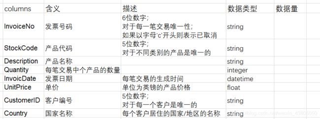
四、数据清洗
import pandas as pd;
import numpy as np;
import datetime as dt;

# for visualization
%pylab
%matplotlib inline
import matplotlib.pyplot as plt
import seaborn as sns

# for machine learning algorithm
from sklearn.preprocessing import StandardScaler
from sklearn.cluster import KMeans

import warnings
warnings.filterwarnings('ignore')
warnings.simplefilter('ignore')
fileNameStr='C:/Users/10138/Desktop/data_analysis/python_data_analysis/电商数据实战/Online Retail.xlsx'
ORdata = pd.read_excel(fileNameStr)
ORdata.head()
| InvoiceNo | StockCode | Description | Quantity | InvoiceDate | UnitPrice | CustomerID | Country | |
|---|---|---|---|---|---|---|---|---|
| 0 | 536365 | 85123A | WHITE HANGING HEART T-LIGHT HOLDER | 6 | 2010-12-01 08:26:00 | 2.55 | 17850.0 | United Kingdom |
| 1 | 536365 | 71053 | WHITE METAL LANTERN | 6 | 2010-12-01 08:26:00 | 3.39 | 17850.0 | United Kingdom |
| 2 | 536365 | 84406B | CREAM CUPID HEARTS COAT HANGER | 8 | 2010-12-01 08:26:00 | 2.75 | 17850.0 | United Kingdom |
| 3 | 536365 | 84029G | KNITTED UNION FLAG HOT WATER BOTTLE | 6 | 2010-12-01 08:26:00 | 3.39 | 17850.0 | United Kingdom |
| 4 | 536365 | 84029E | RED WOOLLY HOTTIE WHITE HEART. | 6 | 2010-12-01 08:26:00 | 3.39 | 17850.0 | United Kingdom |
一、 数据清洗
1.1 查看数据基本信息
ORdata.info()
RangeIndex: 541909 entries, 0 to 541908
Data columns (total 8 columns):
 #   Column       Non-Null Count   Dtype
---  ------       --------------   -----
 0   InvoiceNo    541909 non-null  object
 1   StockCode    541909 non-null  object
 2   Description  540455 non-null  object
 3   Quantity     541909 non-null  int64
 4   InvoiceDate  541909 non-null  datetime64[ns]
 5   UnitPrice    541909 non-null  float64
 6   CustomerID   406829 non-null  float64
 7   Country      541909 non-null  object
dtypes: datetime64[ns](1), float64(2), int64(1), object(4)
memory usage: 33.1+ MB
ORdata.describe()
| Quantity | UnitPrice | CustomerID | |
|---|---|---|---|
| count | 541909.000000 | 541909.000000 | 406829.000000 |
| mean | 9.552250 | 4.611114 | 15287.690570 |
| std | 218.081158 | 96.759853 | 1713.600303 |
| min | -80995.000000 | -11062.060000 | 12346.000000 |
| 25% | 1.000000 | 1.250000 | 13953.000000 |
| 50% | 3.000000 | 2.080000 | 15152.000000 |
| 75% | 10.000000 | 4.130000 | 16791.000000 |
| max | 80995.000000 | 38970.000000 | 18287.000000 |
1.2 缺失值处理
ORdata.isnull().sum()
InvoiceNo           0
StockCode           0
Description      1454
Quantity            0
InvoiceDate         0
UnitPrice           0
CustomerID     135080
Country             0
dtype: int64
将description和customerID存在缺失值,直接做删除处理
ORdata = ORdata.dropna()
ORdata.info()
Int64Index: 406829 entries, 0 to 541908
Data columns (total 8 columns):
 #   Column       Non-Null Count   Dtype
---  ------       --------------   -----
 0   InvoiceNo    406829 non-null  object
 1   StockCode    406829 non-null  object
 2   Description  406829 non-null  object
 3   Quantity     406829 non-null  int64
 4   InvoiceDate  406829 non-null  datetime64[ns]
 5   UnitPrice    406829 non-null  float64
 6   CustomerID   406829 non-null  float64
 7   Country      406829 non-null  object
dtypes: datetime64[ns](1), float64(2), int64(1), object(4)
memory usage: 27.9+ MB
1.3 重复值删除
ORdataUni = ORdata.drop_duplicates()
ORdata.shape[0]-ORdataUni.shape[0]
5225
一共删除了5225条重复值
1.4 异常值处理
ORdataUni.describe()
| Quantity | UnitPrice | CustomerID | |
|---|---|---|---|
| count | 401604.000000 | 401604.000000 | 401604.000000 |
| mean | 12.183273 | 3.474064 | 15281.160818 |
| std | 250.283037 | 69.764035 | 1714.006089 |
| min | -80995.000000 | 0.000000 | 12346.000000 |
| 25% | 2.000000 | 1.250000 | 13939.000000 |
| 50% | 5.000000 | 1.950000 | 15145.000000 |
| 75% | 12.000000 | 3.750000 | 16784.000000 |
| max | 80995.000000 | 38970.000000 | 18287.000000 |
quantity指的是购买的数量,不可能存在负数;UnitPrice是单价,不可能存在负值。将异常值直接删除。
saleOR = ORdataUni.loc[(ORdataUni['Quantity']>0) & (ORdataUni['UnitPrice']>0)]
二、RFM模型寻找价值用户
使用RFM模型对用户进行分类,根据用户分类可以进行精细化运营。
RFM主要的三个指标:
R(Recency) 最近一次消费时间:用户最近一次购买到现在的时间间隔;Recency越短越有价值
F(Frequency) 消费频率:用户在特定时间段内的购买次数;次数越多越有价值
M(Monetary) 消费金额:用户在特定时期的消费总金额;金额越大越有价值
2.1 R,F,M 指标计算
# 统计中的购买日期是范围是2011-01-18到2011-12-02
# R值定义为 最近一次购买日期 距离 2011-12-03 的时间间隔

saleOR['CustomerID']=saleOR['CustomerID'].apply(lambda x:int(x))
Nowdate = saleOR.InvoiceDate.max()+dt.timedelta(days=1)
saleOR = saleOR.drop_duplicates(subset=['InvoiceNo'])

saleOR['TotalSum'] = saleOR['UnitPrice']*saleOR['Quantity']
saleOR.head()
| InvoiceNo | StockCode | Description | Quantity | InvoiceDate | UnitPrice | CustomerID | Country | TotalSum | |
|---|---|---|---|---|---|---|---|---|---|
| 0 | 536365 | 85123A | WHITE HANGING HEART T-LIGHT HOLDER | 6 | 2010-12-01 08:26:00 | 2.55 | 17850 | United Kingdom | 15.30 |
| 7 | 536366 | 22633 | HAND WARMER UNION JACK | 6 | 2010-12-01 08:28:00 | 1.85 | 17850 | United Kingdom | 11.10 |
| 9 | 536367 | 84879 | ASSORTED COLOUR BIRD ORNAMENT | 32 | 2010-12-01 08:34:00 | 1.69 | 13047 | United Kingdom | 54.08 |
| 21 | 536368 | 22960 | JAM MAKING SET WITH JARS | 6 | 2010-12-01 08:34:00 | 4.25 | 13047 | United Kingdom | 25.50 |
| 25 | 536369 | 21756 | BATH BUILDING BLOCK WORD | 3 | 2010-12-01 08:35:00 | 5.95 | 13047 | United Kingdom | 17.85 |
建立用户数据表,每一行代表一个用户的信息
CusDate = saleOR.groupby(['CustomerID']).agg({
     'InvoiceDate':lambda x:(Nowdate-x.max()).days,
                                    'InvoiceNo':'count',
                                    'TotalSum':'sum'}).reset_index()

CusDate.rename(columns={
     'InvoiceDate':'Recency','InvoiceNo':'Frequency','TotalSum':'MonetaryValue'}
           ,inplace= True)
CusDate['Recency'] = CusDate['Recency'].map(lambda x:round(x/30,2))
CusDate.head()
| CustomerID | Recency | Frequency | MonetaryValue | |
|---|---|---|---|---|
| 0 | 12346 | 10.87 | 1 | 77183.60 |
| 1 | 12347 | 0.07 | 7 | 163.16 |
| 2 | 12348 | 2.50 | 4 | 331.36 |
| 3 | 12349 | 0.63 | 1 | 15.00 |
| 4 | 12350 | 10.33 | 1 | 25.20 |
2.2 查看R,F,M 指标分布
呈现R,F,M值的分布情况,以便后续对RFM进行高低维度划分提供依据
R分布
CusDate['Recency'].describe()
count    4338.000000
mean        3.084514
std         3.333842
min         0.030000
25%         0.600000
50%         1.700000
75%         4.730000
max        12.470000
Name: Recency, dtype: float64
# 切片情况呈现
# 每隔一个月作为一个区间
bins_R = np.arange(13)
pd.cut(CusDate['Recency'],bins_R).value_counts()
(0, 1]      1648
(1, 2]       748
(2, 3]       493
(3, 4]       232
(5, 6]       181
(4, 5]       176
(8, 9]       163
(7, 8]       156
(6, 7]       155
(9, 10]      118
(10, 11]     117
(11, 12]      59
Name: Recency, dtype: int64
import matplotlib.pyplot as plt
%pylab
%matplotlib inline
pd.cut(CusDate['Recency'],bins_R,right=False).value_counts().plot.bar()

F分布
CusDate['Frequency'].describe()
count    4338.000000
mean        4.272015
std         7.697998
min         1.000000
25%         1.000000
50%         2.000000
75%         5.000000
max       209.000000
Name: Frequency, dtype: float64
m = np.arange(211)
bins_F= m[::10]
pd.cut(CusDate['Frequency'], bins_F,right=False).value_counts().plot.bar()

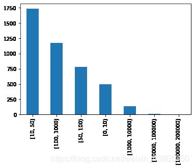
M分布
CusDate['MonetaryValue'].describe()
count      4338.000000
mean        296.914539
std        3128.698664
min           0.390000
25%          17.700000
50%          47.050000
75%         130.102500
max      168471.250000
Name: MonetaryValue, dtype: float64
bins_M = [0,10,50,100,1000,10000,100000,200000]
pd.cut(CusDate['MonetaryValue'],bins_M,right=False).value_counts()
[10, 50)            1736
[100, 1000)         1172
[50, 100)            784
[0, 10)              496
[1000, 10000)        137
[10000, 100000)       12
[100000, 200000)       1
Name: MonetaryValue, dtype: int64
pd.cut(CusDate['MonetaryValue'],bins_M,right=False).value_counts().plot.bar()
2.3 RFM模型搭建(方法一)
分别计算三个指标的中位数,每个指标与中位数进行比较,划分高低,一共会得到8组分类
为每一个用户的R,F,M值进行高低维度的划分;高用‘H’表示,低用‘L’表示。高与低是针对用户值的高低而言的。
R值若小于中位数,则为高,否则为低
F值若大于中位数,则为高,否则为低
M值若大于中位数,则为高,否则为低
R_median = CusDate['Recency'].median()
CusDate['R_label'] = pd.cut(CusDate['Recency'],bins=[0,R_median,CusDate['Recency'].max()+1],right=False
                                ,labels=['H','L'])
CusDate.groupby(['R_label'])['CustomerID'].count()
R_label
H    2158
L    2180
Name: CustomerID, dtype: int64
F_median = CusDate['Frequency'].median()
CusDate['F_label'] = pd.cut(CusDate['Frequency'],bins=[0,F_median,CusDate['Frequency'].max()+1],
                            right=False,labels=['L','H'])
CusDate.groupby(['F_label'])['CustomerID'].count()
F_label
L    1493
H    2845
Name: CustomerID, dtype: int64
M_median = CusDate['MonetaryValue'].median()
CusDate['M_label'] = pd.cut(CusDate['MonetaryValue'],bins=[0,M_median,CusDate['MonetaryValue'].max()+1],
                            right=False,labels=['L','H'])
CusDate.groupby(['M_label'])['CustomerID'].count()
M_label
L    2169
H    2169
Name: CustomerID, dtype: int64
CusDate.head()
| CustomerID | Recency | Frequency | MonetaryValue | R_label | F_label | M_label | |
|---|---|---|---|---|---|---|---|
| 0 | 12346 | 10.87 | 1 | 77183.60 | L | L | H |
| 1 | 12347 | 0.07 | 7 | 163.16 | H | H | H |
| 2 | 12348 | 2.50 | 4 | 331.36 | L | H | H |
| 3 | 12349 | 0.63 | 1 | 15.00 | H | L | L |
| 4 | 12350 | 10.33 | 1 | 25.20 | L | L | L |
def add_rfm(x):
    return str(x['R_label'])+str(x['F_label'])+str(x['M_label'])
CusDate['RFM_label'] = CusDate.apply(add_rfm, axis =1)
CusDate.head()
| CustomerID | Recency | Frequency | MonetaryValue | R_label | F_label | M_label | RFM_label | |
|---|---|---|---|---|---|---|---|---|
| 0 | 12346 | 10.87 | 1 | 77183.60 | L | L | H | LLH |
| 1 | 12347 | 0.07 | 7 | 163.16 | H | H | H | HHH |
| 2 | 12348 | 2.50 | 4 | 331.36 | L | H | H | LHH |
| 3 | 12349 | 0.63 | 1 | 15.00 | H | L | L | HLL |
| 4 | 12350 | 10.33 | 1 | 25.20 | L | L | L | LLL |
用户分类结果
CusDate.groupby(['RFM_label'])['CustomerID'].count()
RFM_label
HHH    1321
HHL     481
HLH      42
HLL     314
LHH     630
LHL     413
LLH     176
LLL     961
Name: CustomerID, dtype: int64
2.4 RFM模型搭建 (方法二)
(1) 将三个指标分别等分 进行打分
(2) 分别计算三个指标 打分 的平均值,每个指标与平均值进行比较,划分高低
(3) 222=8,一共8类数据
R,F,M指标打分
将R,F,M值分别划分为1-4等级,对应1-4分,分数越高,用户价值越高
r_labels=list(range(4,0,-1))
f_labels=list(range(1,5))
m_labels=list(range(1,5,1))
print(list(f_labels))
CusDate['Frequency'].describe()
count    4338.000000
mean        4.272015
std         7.697998
min         1.000000
25%         1.000000
50%         2.000000
75%         5.000000
max       209.000000
Name: Frequency, dtype: float64
CusDate['r_score'] = pd.qcut(CusDate['Recency'],q=4,duplicates='drop',labels=r_labels)
CusDate['f_score'] = pd.qcut(CusDate['Frequency'],q=5,duplicates='drop',labels=f_labels)
CusDate['m_score'] = pd.qcut(CusDate['MonetaryValue'],q=4,duplicates='drop',labels=m_labels)
CusDate['Frequency'].describe()
CusDate['RFM_score'] = CusDate['r_score'].astype('float')+CusDate['f_score'].astype('float')+CusDate['m_score'].astype('float')
mean_R_score = CusDate['r_score'].astype('float').mean()
mean_F_score = CusDate['f_score'].astype('float').mean()
mean_M_score = CusDate['m_score'].astype('float').mean()
print(mean_R_score,mean_F_score,mean_M_score)
2.5138312586445366 1.9709543568464731 2.4972337482710927
R,F,M 高低划分
根据指标分数与总体得分的平均值进行比较,划分高低
CusDate['r_score_label'] = pd.cut(CusDate['r_score'],bins=[0,mean_R_score,5],
                            right=True,labels=['L','H'])  # 左开右毕(0,2.5] (2.5,4])
CusDate['f_score_label'] = pd.cut(CusDate['f_score'],bins=[0,mean_R_score,5],
                            right=True,labels=['L','H'])  # 左开右毕(0,2.5] (2.5,4])
CusDate['m_score_label'] = pd.cut(CusDate['m_score'],bins=[0,mean_M_score,5],
                            right=True,labels=['L','H'])  # 左开右毕(0,2.5] (2.5,4])
def score_label_segment(CusDate):
    return str(CusDate['r_score_label']) +str(CusDate['f_score_label'])+str(CusDate['m_score_label'])
CusDate['RFM_score_label'] = CusDate.apply(score_label_segment,axis=1)
CusDate.head()
| CustomerID | Recency | Frequency | MonetaryValue | R_label | F_label | M_label | RFM_label | r_score | f_score | m_score | RFM_score | r_score_label | f_score_label | m_score_label | RFM_score_label | |
|---|---|---|---|---|---|---|---|---|---|---|---|---|---|---|---|---|
| 0 | 12346 | 10.87 | 1 | 77183.60 | L | L | H | LLH | 1 | 1 | 4 | 6.0 | L | L | H | LLH |
| 1 | 12347 | 0.07 | 7 | 163.16 | H | H | H | HHH | 4 | 4 | 4 | 12.0 | H | H | H | HHH |
| 2 | 12348 | 2.50 | 4 | 331.36 | L | H | H | LHH | 2 | 3 | 4 | 9.0 | L | H | H | LHH |
| 3 | 12349 | 0.63 | 1 | 15.00 | H | L | L | HLL | 3 | 1 | 1 | 5.0 | H | L | L | HLL |
| 4 | 12350 | 10.33 | 1 | 25.20 | L | L | L | LLL | 1 | 1 | 2 | 4.0 | L | L | L | LLL |
两种求解RFM模型的方法比较
方法一:
CusDate.groupby(['RFM_label'])['CustomerID'].count()
RFM_label
HHH    1321
HHL     481
HLH      42
HLL     314
LHH     630
LHL     413
LLH     176
LLL     961
Name: CustomerID, dtype: int64
方法二:
CusDate.groupby(['RFM_score_label'])['CustomerID'].count()
RFM_score_label
HHH    1075
HHL     102
HLH     303
HLL     708
LHH     286
LHL      39
LLH     505
LLL    1320
Name: CustomerID, dtype: int64
CusDate.groupby(['RFM_score_label'])['RFM_score'].mean()
RFM_score_label
HHH    10.861395
HHL     8.539216
HLH     8.161716
HLL     6.026836
LHH     8.604895
LHL     6.461538
LLH     6.138614
LLL     3.930303
Name: RFM_score, dtype: float64
上述两种方法想比较可知:分类之后每一类别的用户数量是有较大差异的。方法二由于选择平均值划分高低,而数据存在左偏现象。所以类别间用户数差异明显。LHL和HHL组内分别只有6人和10人,不能为用户分析提供价值。而方法一得到的用户分群结果相对更合理。
因此,在数量量严重倾斜时,选择中位数作为评判的标准,可行性是更高的。
对于模型好坏的评价标准,更应该结合业务进行评判。
三、K-means聚类寻找价值用户
RFM = CusDate[['CustomerID','Recency','Frequency','MonetaryValue']]
RFM.describe()
| CustomerID | Recency | Frequency | MonetaryValue | |
|---|---|---|---|---|
| count | 4338.000000 | 4338.000000 | 4338.000000 | 4338.000000 |
| mean | 15300.408022 | 3.084514 | 4.272015 | 296.914539 |
| std | 1721.808492 | 3.333842 | 7.697998 | 3128.698664 |
| min | 12346.000000 | 0.030000 | 1.000000 | 0.390000 |
| 25% | 13813.250000 | 0.600000 | 1.000000 | 17.700000 |
| 50% | 15299.500000 | 1.700000 | 2.000000 | 47.050000 |
| 75% | 16778.750000 | 4.730000 | 5.000000 | 130.102500 |
| max | 18287.000000 | 12.470000 | 209.000000 | 168471.250000 |
3.1 选择特征值和样本数据
特征值使用R, F, M
import matplotlib.pyplot as plt
import seaborn as sns
%pylab
%matplotlib inline
f,ax = plt.subplots(3,1,figsize=(10, 12))
plt.subplot(3,1,1); sns.distplot(RFM['Recency'],label='Recency')
plt.subplot(3,1,2); sns.distplot(RFM['Frequency'],label='Frequency')
plt.subplot(3,1,3); sns.distplot(RFM['MonetaryValue'],label='MonetaryValue')

K-means算法对数据的要求:
(1)变量值是对称分布的
(2)变量进行归一化处理,平均值和方差均相同
由R,F,M三个变量的分布图可知,变量值分布不满足对称性,可以使用对数变换解决
3.2 数据预处理
(1) 对数变换
# 将等于0的值替换成1,否则log变换后会出现无穷大的情况,无法使用distplot
RFM.Recency[RFM['Recency']==0]=0.01
RFM.Recency[RFM['Frequency']==0]=0.01
RFM.Recency[RFM['MonetaryValue']==0]=0.01
RFM['Recency'].describe()
RFM_log = RFM[['Recency','Frequency','MonetaryValue']].apply(np.log,axis=1).round(3)
# RFM_log['Recency'].describe()
# RFM['Recency'].describe()
f,ax = plt.subplots(3,1,figsize=(10, 12))
plt.subplot(3,1,1); sns.distplot(RFM_log['Recency'],label='Recency')
plt.subplot(3,1,2); sns.distplot(RFM_log['Frequency'],label='Frequency')
plt.subplot(3,1,3); sns.distplot(RFM_log['MonetaryValue'],label='MonetaryValue')

(2) 标准化处理
fit() : 得到预处理后的数据,计算矩阵列均值和列标准差
transform(data): 得到标准化的矩阵 ,用此方法,必须使用fit先进行预处理计算均值和标准差
然后用fit计算的均值和标准差,进行标准化处理 {x_i - u}/标准差
fit_transform(data) 相当于是fit和transform的组合
from sklearn.preprocessing import StandardScaler
scaler = StandardScaler()
scaler.fit(RFM_log)
RFM_normalization = scaler.transform(RFM_log)
3.3 选择聚类数目
通常有两种方法,一是肘部法则(Elbow Criterion method),选择代价函数下降的显著转折点; 二是业务经验
这里使用肘部法则进行K值选择,并且使用Calinski-Harabasz Index进行评估
from sklearn.cluster import KMeans
# k值的选择,1~8
ks = range(1,9)
inertias=[]
for k in  ks:
    kc = KMeans(n_clusters=k, init='k-means++', random_state = 1)
    kc.fit(RFM_normalization)
    inertias.append(kc.inertia_) # 样本距离其聚类中心的距离平方和

    print('k=',k,' 迭代次数',kc.n_iter_)
k= 1  迭代次数 2
k= 2  迭代次数 8
k= 3  迭代次数 19
k= 4  迭代次数 61
k= 5  迭代次数 21
k= 6  迭代次数 30
k= 7  迭代次数 96
k= 8  迭代次数 24
绘制每个K值对应的inertia_
f,ax = subplots(figsize=(10,6))
plt.plot(ks, inertias,'-o')
plt.xlabel('Number of clusters')
plt.ylabel('Sum of squared distances')
plt.title('Elbow Criterion method to find best k')

根据肘部法则定理,可以看到当k=2,3时,代价函数下降会有一个显著转折点。计算K=2和K=3时Calinski-Harabasz Index对应的值
from sklearn import metrics
kk = range(2,9)
for k in kk:
    y_pred = KMeans(n_clusters=k, random_state=1).fit_predict(RFM_normalization) #k必须大于1
    calinski = metrics.calinski_harabaz_score(RFM_normalization, y_pred)
    print('k:',k,'   calinski=',calinski)
k: 2    calinski= 3850.5792408991447
k: 3    calinski= 3111.8628177429787
k: 4    calinski= 2821.93334700249
k: 5    calinski= 2619.693743897193
k: 6    calinski= 2521.071800973828
k: 7    calinski= 2437.0066461847027
k: 8    calinski= 2329.96118662267
k=2时,calinski_harabaz_scores是最大的,其次是k=3。结合业务而言,如果将用户分成两类,精确度不够高,因此接下来选择k=3进行接下来的验证
3.4 模型计算
kc = KMeans(n_clusters=3, random_state=1)
kc.fit(RFM_normalization)
#  每个样本对应的类簇标签,顺序与样本原始顺序一致
cluster_label = kc.labels_
RFM['K-means_label'] = cluster_label
RFM.head()
| CustomerID | Recency | Frequency | MonetaryValue | K-means_label | |
|---|---|---|---|---|---|
| 0 | 12346 | 10.87 | 1 | 77183.60 | 1 |
| 1 | 12347 | 0.07 | 7 | 163.16 | 2 |
| 2 | 12348 | 2.50 | 4 | 331.36 | 1 |
| 3 | 12349 | 0.63 | 1 | 15.00 | 0 |
| 4 | 12350 | 10.33 | 1 | 25.20 | 0 |
RFM.head()
| CustomerID | Recency | Frequency | MonetaryValue | K-means_label | |
|---|---|---|---|---|---|
| 0 | 12346 | 10.87 | 1 | 77183.60 | 1 |
| 1 | 12347 | 0.07 | 7 | 163.16 | 2 |
| 2 | 12348 | 2.50 | 4 | 331.36 | 1 |
| 3 | 12349 | 0.63 | 1 | 15.00 | 0 |
| 4 | 12350 | 10.33 | 1 | 25.20 | 0 |
3.5 组内特征
RFM.groupby(['K-means_label']).agg({
     'Recency':'mean','Frequency':'mean','MonetaryValue':['mean','count']})
| Recency | Frequency | MonetaryValue | ||
|---|---|---|---|---|
| mean | mean | mean | count | |
| K-means_label | ||||
| 0 | 5.323421 | 1.238681 | 24.145847 | 1789 |
| 1 | 2.014286 | 3.456446 | 171.681266 | 1722 |
| 2 | 0.469674 | 12.532044 | 1147.742696 | 827 |
对于RFM模型而言,R越小越好,而F和M则越大越好。因此,类别2的群体是最有价值的用户群体。
除了每位顾客的R,F,M信息之外,Country也是一个重要的特征描述
# 将原始数据的country信息合并到RFM表格中
saleOR_country = saleOR.drop_duplicates(subset=['CustomerID','Country'])
Customer_feature = pd.merge(left = RFM, right =saleOR_country[['CustomerID','Country']],
                            left_on='CustomerID', right_on='CustomerID',how='left')
Customer_feature.pivot_table(Customer_feature,index = ['K-means_label','Country'],
                             aggfunc='count')['CustomerID']
label02_feature=Customer_feature.loc[Customer_feature['K-means_label']==2,:].groupby(['Country']).count()
label02_feature.sort_values('CustomerID',ascending=False)
#United Kingdom 1625人

label01_feature=Customer_feature.loc[Customer_feature['K-means_label']==1,:].groupby(['Country']).count()
label01_feature.sort_values('CustomerID',ascending=False)
#United Kingdom 1568人

label00_feature=Customer_feature.loc[Customer_feature['K-means_label']==0,:].groupby(['Country']).count()
label00_feature.sort_values('CustomerID',ascending=False);
#United Kingdom 727人
对标签为0,1,2的三类用户分别查看所属国家信息,发现来自United Kingdom的比例分别是16.8%, 36.2%, 37.4%。
来自英国的人数总占比为90.4%,国家这一特征对于三类用户而言并没有明显的差异性
不同组内的用户特征总结:
类别00的用户群体:占总人群的41.2%。Recency,Frequency, MonetrryValue的平均值分别为5.3,1.2,24.1
类别01的用户群体:占总人群的39.7%。Recency,Frequency, MonetrryValue的平均值分别为2.0,3.5,171.7
类别02的用户群体:占总人群的19.0%。Recency,Frequency, MonetrryValue的平均值分别为0.5,12.5,1147.8
由此可见,类别02群体是价值最高的用户群体。可以对类别02的用户群体采取重点跟进维系措施。
总结
本次分析主要使用Python语言对来自在英国注册的电子零售企业的交易数据进行数据挖掘。使用传统的RFM模型和K-Means聚类技术分析对电子零售业用户进行分层,寻找有价值的用户。
两种技术得出的结论有所差别,需要业务专家结合具体的应用场景来进行衡量用户分层结果。但是这次分析结果为后期的用户精细化运营提供数据支持,有一定的参考借鉴作用。