基于Keras实现电影评论文本分类与RNN实现

notebook使用评论文本将影评分为积极（positive）或消极（nagetive）两类。这是一个二元（binary）或者二分类问题，一种重要且应用广泛的机器学习问题。

使用来源于网络电影数据库（Internet Movie Database）的 IMDB 数据集（IMDB dataset），其包含 50,000 条影评文本。从该数据集切割出的25,000条评论用作训练，另外 25,000 条用作测试。训练集与测试集是平衡的（balanced），意味着它们包含相等数量的积极和消极评论。

import tensorflow as tf
from tensorflow import keras

import numpy as np

print(tf.__version__)

结果：

2.3.0

下载 IMDB 数据集

IMDB 数据集已经打包在 Tensorflow 中。该数据集已经经过预处理，评论（单词序列）已经被转换为整数序列，其中每个整数表示字典中的特定单词。

以下代码将下载 IMDB 数据集到您的机器上（如果您已经下载过将从缓存中复制）：

imdb = keras.datasets.imdb

(train_data, train_labels), (test_data, test_labels) = imdb.load_data(num_words=10000)

结果：

Downloading data from https://storage.googleapis.com/tensorflow/tf-keras-datasets/imdb.npz
17465344/17464789 [==============================] - 0s 0us/step

参数 num_words=10000 保留了训练数据中最常出现的 10,000 个单词。为了保持数据规模的可管理性，低频词将被丢弃。

探索数据

让我们花一点时间来了解数据格式。该数据集是经过预处理的：每个样本都是一个表示影评中词汇的整数数组。每个标签都是一个值为 0 或 1 的整数值，其中 0 代表消极评论，1 代表积极评论。

print("Training entries: {}, labels: {}".format(len(train_data), len(train_labels)))

结果：

Training entries: 25000, labels: 25000


评论文本被转换为整数值，其中每个整数代表词典中的一个单词。首条评论是这样的：

print(train_data[0])

结果：

[1, 14, 22, 16, 43, 530, 973, 1622, 1385, 65, 458, 4468, 66, 3941, 4, 173, 36, 256, 5, 25, 100, 43, 838, 112, 50, 670, 2, 9, 35, 480, 284, 5, 150, 4, 172, 112, 167, 2, 336, 385, 39, 4, 172, 4536, 1111, 17, 546, 38, 13, 447, 4, 192, 50, 16, 6, 147, 2025, 19, 14, 22, 4, 1920, 4613, 469, 4, 22, 71, 87, 12, 16, 43, 530, 38, 76, 15, 13, 1247, 4, 22, 17, 515, 17, 12, 16, 626, 18, 2, 5, 62, 386, 12, 8, 316, 8, 106, 5, 4, 2223, 5244, 16, 480, 66, 3785, 33, 4, 130, 12, 16, 38, 619, 5, 25, 124, 51, 36, 135, 48, 25, 1415, 33, 6, 22, 12, 215, 28, 77, 52, 5, 14, 407, 16, 82, 2, 8, 4, 107, 117, 5952, 15, 256, 4, 2, 7, 3766, 5, 723, 36, 71, 43, 530, 476, 26, 400, 317, 46, 7, 4, 2, 1029, 13, 104, 88, 4, 381, 15, 297, 98, 32, 2071, 56, 26, 141, 6, 194, 7486, 18, 4, 226, 22, 21, 134, 476, 26, 480, 5, 144, 30, 5535, 18, 51, 36, 28, 224, 92, 25, 104, 4, 226, 65, 16, 38, 1334, 88, 12, 16, 283, 5, 16, 4472, 113, 103, 32, 15, 16, 5345, 19, 178, 32]

电影评论可能具有不同的长度。以下代码显示了第一条和第二条评论的中单词数量。由于神经网络的输入必须是统一的长度，我们稍后需要解决这个问题。

len(train_data[0]), len(train_data[1])

结果：

(218, 189)

将整数转换回单词

了解如何将整数转换回文本对您可能是有帮助的。这里我们将创建一个辅助函数来查询一个包含了整数到字符串映射的字典对象：

# 一个映射单词到整数索引的词典
word_index = imdb.get_word_index()

# 保留第一个索引
word_index = {k:(v+3) for k,v in word_index.items()}
word_index[""] = 0
word_index[""] = 1
word_index[""] = 2  # unknown
word_index[""] = 3

reverse_word_index = dict([(value, key) for (key, value) in word_index.items()])

def decode_review(text):
    return ' '.join([reverse_word_index.get(i, '?') for i in text])

 

Downloading data from https://storage.googleapis.com/tensorflow/tf-keras-datasets/imdb_word_index.json
1646592/1641221 [==============================] - 0s 0us/step

现在可以使用 decode_review 函数来显示首条评论的文本：

decode_review(train_data[0])

" this film was just brilliant casting location scenery story direction everyone's really suited the part they played and you could just imagine being there robert is an amazing actor and now the same being director father came from the same scottish island as myself so i loved the fact there was a real connection with this film the witty remarks throughout the film were great it was just brilliant so much that i bought the film as soon as it was released for and would recommend it to everyone to watch and the fly fishing was amazing really cried at the end it was so sad and you know what they say if you cry at a film it must have been good and this definitely was also to the two little boy's that played the of norman and paul they were just brilliant children are often left out of the list i think because the stars that play them all grown up are such a big profile for the whole film but these children are amazing and should be praised for what they have done don't you think the whole story was so lovely because it was true and was someone's life after all that was shared with us all"

 

准备数据

影评——即整数数组必须在输入神经网络之前转换为张量。这种转换可以通过以下两种方式来完成：

• 将数组转换为表示单词出现与否的由 0 和 1 组成的向量，类似于 one-hot 编码。例如，序列[3, 5]将转换为一个 10,000 维的向量，该向量除了索引为 3 和 5 的位置是 1 以外，其他都为 0。然后，将其作为网络的首层——一个可以处理浮点型向量数据的稠密层。不过，这种方法需要大量的内存，需要一个大小为 num_words * num_reviews 的矩阵。

• 或者，我们可以填充数组来保证输入数据具有相同的长度，然后创建一个大小为 max_length * num_reviews 的整型张量。我们可以使用能够处理此形状数据的嵌入层作为网络中的第一层。

例如用第二种方法：

由于电影评论长度必须相同，我们将使用 pad_sequences 函数来使长度标准化：

train_data = keras.preprocessing.sequence.pad_sequences(train_data,
                                                        value=word_index[""],
                                                        padding='post',
                                                        maxlen=256)

test_data = keras.preprocessing.sequence.pad_sequences(test_data,
                                                       value=word_index[""],
                                                       padding='post',
                                                       maxlen=256)

样本的长度：

len(train_data[0]), len(train_data[1])

(256, 256)

并检查一下首条评论（当前已经填充）：

print(train_data[0])

[ 1 14 22 16 43 530 973 1622 1385 65 458 4468 66 3941 4 173 36 256 5 25 100 43 838 112 50 670 2 9 35 480 284 5 150 4 172 112 167 2 336 385 39 4 172 4536 1111 17 546 38 13 447 4 192 50 16 6 147 2025 19 14 22 4 1920 4613 469 4 22 71 87 12 16 43 530 38 76 15 13 1247 4 22 17 515 17 12 16 626 18 2 5 62 386 12 8 316 8 106 5 4 2223 5244 16 480 66 3785 33 4 130 12 16 38 619 5 25 124 51 36 135 48 25 1415 33 6 22 12 215 28 77 52 5 14 407 16 82 2 8 4 107 117 5952 15 256 4 2 7 3766 5 723 36 71 43 530 476 26 400 317 46 7 4 2 1029 13 104 88 4 381 15 297 98 32 2071 56 26 141 6 194 7486 18 4 226 22 21 134 476 26 480 5 144 30 5535 18 51 36 28 224 92 25 104 4 226 65 16 38 1334 88 12 16 283 5 16 4472 113 103 32 15 16 5345 19 178 32 0 0 0 0 0 0 0 0 0 0 0 0 0 0 0 0 0 0 0 0 0 0 0 0 0 0 0 0 0 0 0 0 0 0 0 0 0 0]

 

构建模型

神经网络由堆叠的层来构建，这需要从两个主要方面来进行体系结构决策：

• 模型里有多少层？
• 每个层里有多少隐层单元（hidden units）？

在此样本中，输入数据包含一个单词索引的数组。要预测的标签为 0 或 1。让我们来为该问题构建一个模型：

# 输入形状是用于电影评论的词汇数目（10,000 词）
vocab_size = 10000

model = keras.Sequential()
model.add(keras.layers.Embedding(vocab_size, 16))
model.add(keras.layers.GlobalAveragePooling1D())
model.add(keras.layers.Dense(16, activation='relu'))
model.add(keras.layers.Dense(1, activation='sigmoid'))

model.summary()

 

Model: "sequential"
_________________________________________________________________
Layer (type)                 Output Shape              Param #   
=================================================================
embedding (Embedding)        (None, None, 16)          160000    
_________________________________________________________________
global_average_pooling1d (Gl (None, 16)                0         
_________________________________________________________________
dense (Dense)                (None, 16)                272       
_________________________________________________________________
dense_1 (Dense)              (None, 1)                 17        
=================================================================
Total params: 160,289
Trainable params: 160,289
Non-trainable params: 0
_________________________________________________________________

 

层按顺序堆叠以构建分类器：

1. 第一层是嵌入（Embedding）层。该层采用整数编码的词汇表，并查找每个词索引的嵌入向量（embedding vector）。这些向量是通过模型训练学习到的。向量向输出数组增加了一个维度。得到的维度为：(batch, sequence, embedding)。
2. 接下来，GlobalAveragePooling1D 将通过对序列维度求平均值来为每个样本返回一个定长输出向量。这允许模型以尽可能最简单的方式处理变长输入。
3. 该定长输出向量通过一个有 16 个隐层单元的全连接（Dense）层传输。
4. 最后一层与单个输出结点密集连接。使用 Sigmoid 激活函数，其函数值为介于 0 与 1 之间的浮点数，表示概率或置信度。

隐层单元

上述模型在输入输出之间有两个中间层或“隐藏层”。输出（单元，结点或神经元）的数量即为层表示空间的维度。换句话说，是学习内部表示时网络所允许的自由度。

如果模型具有更多的隐层单元（更高维度的表示空间）和/或更多层，则可以学习到更复杂的表示。但是，这会使网络的计算成本更高，并且可能导致学习到不需要的模式——一些能够在训练数据上而不是测试数据上改善性能的模式。这被称为过拟合（overfitting），我们稍后会对此进行探究。

损失函数与优化器

一个模型需要损失函数和优化器来进行训练。由于这是一个二分类问题且模型输出概率值（一个使用 sigmoid 激活函数的单一单元层），我们将使用 binary_crossentropy 损失函数。

这不是损失函数的唯一选择，例如，您可以选择 mean_squared_error 。但是，一般来说 binary_crossentropy 更适合处理概率——它能够度量概率分布之间的“距离”，或者在我们的示例中，指的是度量 ground-truth 分布与预测值之间的“距离”。

稍后，当我们研究回归问题（例如，预测房价）时，我们将介绍如何使用另一种叫做均方误差的损失函数。

现在，配置模型来使用优化器和损失函数：

model.compile(optimizer='adam',
              loss='binary_crossentropy',
              metrics=['accuracy'])

 

创建一个验证集

在训练时，我们想要检查模型在未见过的数据上的准确率（accuracy）。通过从原始训练数据中分离 10,000 个样本来创建一个验证集。（为什么现在不使用测试集？我们的目标是只使用训练数据来开发和调整模型，然后只使用一次测试数据来评估准确率（accuracy））。

x_val = train_data[:10000]
partial_x_train = train_data[10000:]

y_val = train_labels[:10000]
partial_y_train = train_labels[10000:]

 

训练模型

以 512 个样本的 mini-batch 大小迭代 40 个 epoch 来训练模型。这是指对 x_train 和 y_train 张量中所有样本的的 40 次迭代。在训练过程中，监测来自验证集的 10,000 个样本上的损失值（loss）和准确率（accuracy）：

history = model.fit(partial_x_train,
                    partial_y_train,
                    epochs=40,
                    batch_size=512,
                    validation_data=(x_val, y_val),
                    verbose=1)

 

Epoch 1/40
30/30 [==============================] - 1s 18ms/step - loss: 0.6924 - accuracy: 0.5173 - val_loss: 0.6911 - val_accuracy: 0.5699
Epoch 2/40
30/30 [==============================] - 0s 10ms/step - loss: 0.6886 - accuracy: 0.5734 - val_loss: 0.6863 - val_accuracy: 0.6309
Epoch 3/40
30/30 [==============================] - 0s 10ms/step - loss: 0.6810 - accuracy: 0.6439 - val_loss: 0.6766 - val_accuracy: 0.7367
Epoch 4/40
30/30 [==============================] - 0s 10ms/step - loss: 0.6667 - accuracy: 0.7411 - val_loss: 0.6595 - val_accuracy: 0.7328
Epoch 5/40
30/30 [==============================] - 0s 10ms/step - loss: 0.6431 - accuracy: 0.7602 - val_loss: 0.6327 - val_accuracy: 0.7677
Epoch 6/40
30/30 [==============================] - 0s 10ms/step - loss: 0.6086 - accuracy: 0.7896 - val_loss: 0.5968 - val_accuracy: 0.7894
Epoch 7/40
30/30 [==============================] - 0s 10ms/step - loss: 0.5654 - accuracy: 0.8147 - val_loss: 0.5550 - val_accuracy: 0.8102
Epoch 8/40
30/30 [==============================] - 0s 10ms/step - loss: 0.5180 - accuracy: 0.8337 - val_loss: 0.5115 - val_accuracy: 0.8230
Epoch 9/40
30/30 [==============================] - 0s 10ms/step - loss: 0.4709 - accuracy: 0.8535 - val_loss: 0.4705 - val_accuracy: 0.8356
Epoch 10/40
30/30 [==============================] - 0s 10ms/step - loss: 0.4269 - accuracy: 0.8655 - val_loss: 0.4342 - val_accuracy: 0.8454
Epoch 11/40
30/30 [==============================] - 0s 10ms/step - loss: 0.3887 - accuracy: 0.8763 - val_loss: 0.4040 - val_accuracy: 0.8545
Epoch 12/40
30/30 [==============================] - 0s 10ms/step - loss: 0.3566 - accuracy: 0.8843 - val_loss: 0.3799 - val_accuracy: 0.8598
Epoch 13/40
30/30 [==============================] - 0s 10ms/step - loss: 0.3299 - accuracy: 0.8911 - val_loss: 0.3608 - val_accuracy: 0.8660
Epoch 14/40
30/30 [==============================] - 0s 10ms/step - loss: 0.3070 - accuracy: 0.8975 - val_loss: 0.3458 - val_accuracy: 0.8702
Epoch 15/40
30/30 [==============================] - 0s 10ms/step - loss: 0.2876 - accuracy: 0.9021 - val_loss: 0.3334 - val_accuracy: 0.8727
Epoch 16/40
30/30 [==============================] - 0s 10ms/step - loss: 0.2708 - accuracy: 0.9073 - val_loss: 0.3234 - val_accuracy: 0.8753
Epoch 17/40
30/30 [==============================] - 0s 10ms/step - loss: 0.2558 - accuracy: 0.9130 - val_loss: 0.3154 - val_accuracy: 0.8773
Epoch 18/40
30/30 [==============================] - 0s 10ms/step - loss: 0.2428 - accuracy: 0.9175 - val_loss: 0.3102 - val_accuracy: 0.8782
Epoch 19/40
30/30 [==============================] - 0s 10ms/step - loss: 0.2308 - accuracy: 0.9214 - val_loss: 0.3032 - val_accuracy: 0.8812
Epoch 20/40
30/30 [==============================] - 0s 10ms/step - loss: 0.2194 - accuracy: 0.9246 - val_loss: 0.2988 - val_accuracy: 0.8818
Epoch 21/40
30/30 [==============================] - 0s 10ms/step - loss: 0.2093 - accuracy: 0.9280 - val_loss: 0.2956 - val_accuracy: 0.8821
Epoch 22/40
30/30 [==============================] - 0s 10ms/step - loss: 0.2000 - accuracy: 0.9321 - val_loss: 0.2921 - val_accuracy: 0.8838
Epoch 23/40
30/30 [==============================] - 0s 10ms/step - loss: 0.1912 - accuracy: 0.9357 - val_loss: 0.2901 - val_accuracy: 0.8846
Epoch 24/40
30/30 [==============================] - 0s 10ms/step - loss: 0.1829 - accuracy: 0.9396 - val_loss: 0.2885 - val_accuracy: 0.8847
Epoch 25/40
30/30 [==============================] - 0s 10ms/step - loss: 0.1756 - accuracy: 0.9439 - val_loss: 0.2874 - val_accuracy: 0.8844
Epoch 26/40
30/30 [==============================] - 0s 10ms/step - loss: 0.1681 - accuracy: 0.9465 - val_loss: 0.2864 - val_accuracy: 0.8855
Epoch 27/40
30/30 [==============================] - 0s 10ms/step - loss: 0.1617 - accuracy: 0.9481 - val_loss: 0.2867 - val_accuracy: 0.8844
Epoch 28/40
30/30 [==============================] - 0s 10ms/step - loss: 0.1548 - accuracy: 0.9519 - val_loss: 0.2865 - val_accuracy: 0.8861
Epoch 29/40
30/30 [==============================] - 0s 10ms/step - loss: 0.1485 - accuracy: 0.9543 - val_loss: 0.2872 - val_accuracy: 0.8849
Epoch 30/40
30/30 [==============================] - 0s 10ms/step - loss: 0.1426 - accuracy: 0.9561 - val_loss: 0.2881 - val_accuracy: 0.8854
Epoch 31/40
30/30 [==============================] - 0s 10ms/step - loss: 0.1372 - accuracy: 0.9587 - val_loss: 0.2895 - val_accuracy: 0.8851
Epoch 32/40
30/30 [==============================] - 0s 10ms/step - loss: 0.1320 - accuracy: 0.9609 - val_loss: 0.2899 - val_accuracy: 0.8856
Epoch 33/40
30/30 [==============================] - 0s 10ms/step - loss: 0.1267 - accuracy: 0.9625 - val_loss: 0.2911 - val_accuracy: 0.8851
Epoch 34/40
30/30 [==============================] - 0s 10ms/step - loss: 0.1219 - accuracy: 0.9649 - val_loss: 0.2931 - val_accuracy: 0.8851
Epoch 35/40
30/30 [==============================] - 0s 10ms/step - loss: 0.1173 - accuracy: 0.9666 - val_loss: 0.2948 - val_accuracy: 0.8863
Epoch 36/40
30/30 [==============================] - 0s 10ms/step - loss: 0.1127 - accuracy: 0.9685 - val_loss: 0.2985 - val_accuracy: 0.8851
Epoch 37/40
30/30 [==============================] - 0s 10ms/step - loss: 0.1086 - accuracy: 0.9688 - val_loss: 0.2998 - val_accuracy: 0.8860
Epoch 38/40
30/30 [==============================] - 0s 10ms/step - loss: 0.1045 - accuracy: 0.9716 - val_loss: 0.3033 - val_accuracy: 0.8839
Epoch 39/40
30/30 [==============================] - 0s 10ms/step - loss: 0.1007 - accuracy: 0.9723 - val_loss: 0.3049 - val_accuracy: 0.8847
Epoch 40/40
30/30 [==============================] - 0s 10ms/step - loss: 0.0967 - accuracy: 0.9737 - val_loss: 0.3087 - val_accuracy: 0.8832

 

评估模型

我们来看一下模型的性能如何。将返回两个值。损失值（loss）（一个表示误差的数字，值越低越好）与准确率（accuracy）。

results = model.evaluate(test_data,  test_labels, verbose=2)

print(results)

结果：

782/782 - 1s - loss: 0.3298 - accuracy: 0.8729
[0.32977813482284546, 0.8728799819946289]

这种十分朴素的方法得到了约 87% 的准确率（accuracy）。若采用更好的方法，模型的准确率应当接近 95%。

创建一个准确率（accuracy）和损失值（loss）随时间变化的图表

model.fit() 返回一个 History 对象，该对象包含一个字典，其中包含训练阶段所发生的一切事件：

history_dict = history.history
history_dict.keys()

结果：

dict_keys(['loss', 'accuracy', 'val_loss', 'val_accuracy'])

有四个条目：在训练和验证期间，每个条目对应一个监控指标。我们可以使用这些条目来绘制训练与验证过程的损失值（loss）和准确率（accuracy），以便进行比较。

import matplotlib.pyplot as plt

acc = history_dict['accuracy']
val_acc = history_dict['val_accuracy']
loss = history_dict['loss']
val_loss = history_dict['val_loss']

epochs = range(1, len(acc) + 1)

# “bo”代表 "蓝点"
plt.plot(epochs, loss, 'bo', label='Training loss')
# b代表“蓝色实线”
plt.plot(epochs, val_loss, 'b', label='Validation loss')
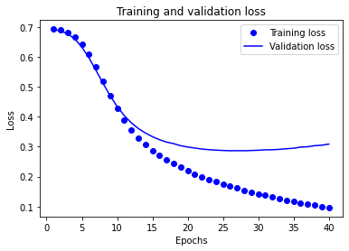
plt.title('Training and validation loss')
plt.xlabel('Epochs')
plt.ylabel('Loss')
plt.legend()

plt.show()

 

plt.clf()   # 清除数字

plt.plot(epochs, acc, 'bo', label='Training acc')
plt.plot(epochs, val_acc, 'b', label='Validation acc')
plt.title('Training and validation accuracy')
plt.xlabel('Epochs')
plt.ylabel('Accuracy')
plt.legend()

plt.show()

 

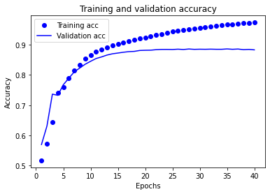
在该图中，点代表训练损失值（loss）与准确率（accuracy），实线代表验证损失值（loss）与准确率（accuracy）。

注意训练损失值随每一个 epoch 下降而训练准确率（accuracy）随每一个 epoch 上升。这在使用梯度下降优化时是可预期的——理应在每次迭代中最小化期望值。

验证过程的损失值（loss）与准确率（accuracy）的情况却并非如此——它们似乎在 20 个 epoch 后达到峰值。这是过拟合的一个实例：模型在训练数据上的表现比在以前从未见过的数据上的表现要更好。在此之后，模型过度优化并学习特定于训练数据的表示，而不能够泛化到测试数据。

 

RNN实现：

import tensorflow_datasets as tfds
import tensorflow as tf
import matplotlib.pyplot as plt

def plot_graphs(history, metric):
    plt.plot(history.history[metric])
    plt.plot(history.history['val_'+metric], '')
    plt.xlabel("Epochs")
    plt.ylabel(metric)
    plt.legend([metric, 'val_'+metric])
    plt.show()

dataset, info = tfds.load('imdb_reviews/subwords8k', with_info=True,as_supervised=True)
train_dataset, test_dataset = dataset['train'], dataset['test']
encoder = info.features['text'].encoder
print('Vocabulary size: {}'.format(encoder.vocab_size))

sample_string = 'Hello TensorFlow.'

encoded_string = encoder.encode(sample_string)
print('Encoded string is {}'.format(encoded_string))

original_string = encoder.decode(encoded_string)
print('The original string: "{}"'.format(original_string))

assert original_string == sample_string
for index in encoded_string:
    print('{} ----> {}'.format(index, encoder.decode([index])))

BUFFER_SIZE = 10000
BATCH_SIZE = 64

train_dataset = train_dataset.shuffle(BUFFER_SIZE)
train_dataset = train_dataset.padded_batch(BATCH_SIZE)

test_dataset = test_dataset.padded_batch(BATCH_SIZE)

model = tf.keras.Sequential([
  tf.keras.layers.Embedding(encoder.vocab_size, 64),
  tf.keras.layers.Bidirectional(tf.keras.layers.LSTM(64)),
  tf.keras.layers.Dense(64, activation='relu'),
  tf.keras.layers.Dense(1)
])

model.compile(loss=tf.keras.losses.BinaryCrossentropy(from_logits=True),
              optimizer=tf.keras.optimizers.Adam(1e-4),
              metrics=['accuracy'])
history = model.fit(train_dataset, epochs=10,
                    validation_data=test_dataset,
                    validation_steps=30)
test_loss, test_acc = model.evaluate(test_dataset)

print('Test Loss: {}'.format(test_loss))
print('Test Accuracy: {}'.format(test_acc))


def pad_to_size(vec, size):
    zeros = [0] * (size - len(vec))
    vec.extend(zeros)
    return vec

def sample_predict(sample_pred_text, pad):
    encoded_sample_pred_text = encoder.encode(sample_pred_text)

    if pad:
      encoded_sample_pred_text = pad_to_size(encoded_sample_pred_text, 64)
    encoded_sample_pred_text = tf.cast(encoded_sample_pred_text, tf.float32)
    predictions = model.predict(tf.expand_dims(encoded_sample_pred_text, 0))

    return (predictions)

sample_pred_text = ('The movie was cool. The animation and the graphics '
                    'were out of this world. I would recommend this movie.')
predictions = sample_predict(sample_pred_text, pad=False)
print(predictions)
# predict on a sample text with padding

sample_pred_text = ('The movie was cool. The animation and the graphics '
                    'were out of this world. I would recommend this movie.')
predictions = sample_predict(sample_pred_text, pad=True)
print(predictions)
plot_graphs(history, 'accuracy')
plot_graphs(history, 'loss')