OpenCV_Python官方文档11——图像阈值

OpenCV-Python Tutorials

https://opencv-python-tutroals.readthedocs.io/en/latest/py_tutorials/py_tutorials.html

阈值（二值化操作），阈值又叫临界值，是指一个效应能够产生的的最低值或最高。

简单阈值

选取一个全局阈值，整个图像都和这个阈值比较，然后就把整幅图像分成了非黑即白的二值图像。

主要函数

ret, dst = cv2.threshold(src, thresh, maxval,type)

• dst： 输出图像
• src： 输入图像，只能输入单通道图像，一般为灰度图
• thresh： 阈值
• maxval： 当像素值大于阈值（或者小于阈值，根据type来决定），所赋予的值
• type：阈值操作的类型
  • cv2.THRESH_BINARY #二元阈值
  • cv2.THRESH_BINARY_INV #逆二元阈值
  • cv2.THRESH_TRUNC
  • cv2.THRESH_TOZERO
  • cv2.THRESH_TOZERO_INV

import cv2
import numpy as np
import matplotlib.pyplot as plt
import os 
os.chdir('C:/Users/lenovo/Pictures/')

img = cv2.imread('butterfly.jpg',0) #读取图片并直接将图像灰度化
ret,thresh1 = cv2.threshold(img,127,255,cv2.THRESH_BINARY) #如果一个像素值低于127，则像素值转换为255（白色色素值），否则转换成0（黑色色素值）
ret,thresh2 = cv2.threshold(img,127,255,cv2.THRESH_BINARY_INV)
ret,thresh3 = cv2.threshold(img,127,255,cv2.THRESH_TRUNC)
ret,thresh4 = cv2.threshold(img,127,255,cv2.THRESH_TOZERO)
ret,thresh5 = cv2.threshold(img,127,255,cv2.THRESH_TOZERO_INV)

titles = ['Original Image','BINARY','BINARY_INV','TRUNC','TOZERO','TOZERP_INV']
imgs = [img,thresh1,thresh2,thresh3,thresh4,thresh5]
for i in range(len(imgs)):
    plt.subplot(2,3,i+1)
    plt.imshow(imgs[i],'gray')
    plt.title(titles[i])
    plt.axis('off')
plt.show()

输出结果：

自适应阈值

局部性阈值，根据图像上的每一个小区域计算与其对应的阀值。通过规定一个区域大小，比较这个点与区域大小里面像素点的平均值（或者其他特征）的大小关系确定该像素点的值。因此在同一幅图像上的不同区域采用的是不同的阀值，从而使我们能在亮度不同的情况下得到更好的结果。

主要函数

dst = cv2.adaptiveThreshold(src, maxval, thresh_type, type, Block Size, C)

• dst： 输出图像
• src： 输入图像，只能输入单通道图像，一般为灰度图
• maxval： 当像素值大于阈值（或者小于阈值，根据type来决定），所赋予的值
• thresh_type： 阈值计算方法
  • cv2.ADAPTIVE_THRESH_MEAN_C #阀值取邻域的平均值
  • cv2.ADAPTIVE_THRESH_GAUSSIAN_C #阀值取邻域的加权和，权重为一个高斯窗口
• type：阈值操作的类型
  • cv2.THRESH_BINARY #二元阈值
  • cv2.THRESH_BINARY_INV #逆二元阈值
  • cv2.THRESH_TRUNC
  • cv2.THRESH_TOZERO
  • cv2.THRESH_TOZERO_INV
• Block Size： 计算阈值的区域大小
• C ：阈值计算方法中的常数项，阈值等于均值或者加权值减去这个常数C

import cv2
import numpy as np
import matplotlib.pyplot as plt
import os 
os.chdir('C:/Users/lenovo/Pictures/')

img = cv2.imread('butterfly.jpg',0) #读取图片并直接将图像灰度化
#中值滤波 起到平滑图像，滤去噪声的作用
img = cv2.medianBlur(img,5)
ret,th1 = cv2.threshold(img,127,255,cv2.THRESH_BINARY) #11为block size，2为C
th2 = cv2.adaptiveThreshold(img,255,cv2.ADAPTIVE_THRESH_MEAN_C,cv2.THRESH_BINARY,11,2)
th3 = cv2.adaptiveThreshold(img,255,cv2.ADAPTIVE_THRESH_GAUSSIAN_C,cv2.THRESH_BINARY,11,2)

titles = ['Original Image','global thresholding(v=127)','Adaptive mean thresholding','Adaptive gaussian thresholding']
imgs = [img,th1,th2,th3]
for i in range(len(imgs)):
    plt.subplot(2,2,i+1)
    plt.imshow(imgs[i],'gray')
    plt.title(titles[i])
    plt.axis('off')
plt.show()

输出结果： 上述阈值区域大小设置为11，当窗口越小，得到的图像越细。

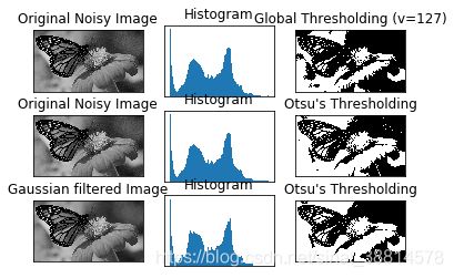
Otsu 二值化

最大类间方差法是由日本学者大津于1979年提出的,是一种自适应的阈值确定的方法,又叫大津法,简称OTSU。

cv2.threshold()是有两个返回值的，前面一直用的第二个返回值，也就是阈值处理后的图像，那么第一个返回值（得到图像的阈值）将会在这里用到。
前面对于阈值的处理上，我们选择的阈值都是127，那么实际情况下，怎么去选择这个127呢？有的图像可能阈值不是127得到的效果更好。那么这里需要算法自己去寻找到一个阈值，而Otsu就可以自己找到一个认为最好的阈值。并且Otsu非常适合于图像灰度直方图具有双峰的情况，他会在双峰之间找到一个值作为阈值，对于非双峰图像，可能并不是很好用。那么经过Otsu得到的那个阈值就是cv2.threshold()的第一个参数了。因为Otsu方法会产生一个阈值，那么函数cv2.threshold()的的第二个参数（设置阈值）就是0了，并且在cv2.threshold()的方法参数中还得加上语句cv2.THRESH_OTSU。

Otsu过程：

1. 计算图像直方图；
2. 设定一阈值，把直方图强度大于阈值的像素分成一组，把小于阈值的像素分成另外一组；
3. 分别计算两组内的偏移数，并把偏移数相加；
4. 把0~255依照顺序多为阈值，重复1-3的步骤，直到得到最小偏移数，其所对应的值即为结果阈值。

绘制直方图

plt.hist(src,pixels)

• src:数据源，注意这里只能传入一维数组，使用src.ravel()可以将二维图像拉平为一维数组。
• pixels:像素级，一般输入256。

import cv2
import numpy as np
import matplotlib.pyplot as plt
import os 
os.chdir('C:/Users/lenovo/Pictures/')

img = cv2.imread('butterfly.jpg',0) #读取图片并直接将图像灰度化

#Global Thresholding
ret1,th1 = cv2.threshold(img,127,255,cv2.THRESH_BINARY)

#Otsu's Thresholding
ret2,th2 = cv2.threshold(img,0,255,cv2.THRESH_BINARY+cv2.THRESH_OTSU)

#Otsu's Thresholding after Gaussian Filtering 高斯滤波
blur = cv2.GaussianBlur(img,(5,5),0) #(5,5)为高斯内核大小,0为标准偏差
ret3,th3 = cv2.threshold(blur,0,255,cv2.THRESH_BINARY+cv2.THRESH_OTSU)#阈值设为0

#plot all the images and their histograms
imgs = [img,0,th1,img,0,th2,blur,0,th3]
titles = ['Original Noisy Image','Histogram','Global Thresholding (v=127)',
          'Original Noisy Image','Histogram',"Otsu's Thresholding",
          'Gaussian filtered Image','Histogram',"Otsu's Thresholding"]
for i in range(3):       
    plt.subplot(3,3,i*3+1),plt.imshow(imgs[i*3],'gray')
    plt.title(titles[i*3]),plt.xticks([]),plt.yticks([])
    plt.subplot(3,3,i*3+2),plt.hist(imgs[i*3].ravel(),256)
    plt.title(titles[i*3+1]), plt.xticks([]), plt.yticks([])
    plt.subplot(3,3,i*3+3),plt.imshow(imgs[i*3+2],'gray')
    plt.title(titles[i*3+2]), plt.xticks([]), plt.yticks([])    
plt.show()
print (ret2)

输出结果： 用Otsu算出的阈值为98