https://bioconductor.org/packages/devel/bioc/vignettes/ggtreeExtra/inst/doc/ggtreeExtra.html
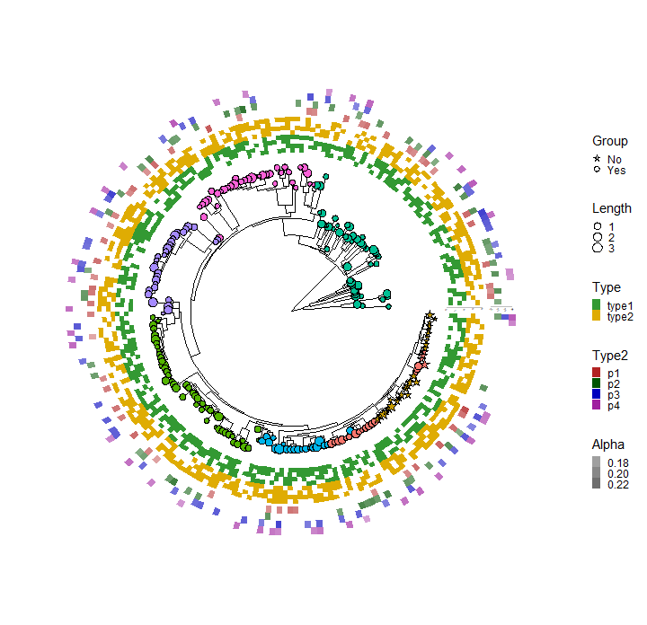
circos画图是基于染色体,按照半径来绘制的。但是进化树并不是基于染色体,基于进化树的圈图,可以添加其他的图层。基于ggtree和ggplot2的进化树圈图包ggtreeExtra可以实现这个功能。Y叔出品,图比较美观。
setwd("e:/bioinformation_center/Rcode/ggtreeExtra")

##目的是画进化树和热图

library(ggtreeExtra)
library(ggstar)
library(ggplot2)
library(ggtree)
library(treeio)
library(ggnewscale)

#BiocManager::install("ggtreeExtra")
library(ggtreeExtra)


# The path of tree file.
trfile <- system.file("extdata", "tree.nwk", package="ggtreeExtra")
# The path of file to plot tippoint.
tippoint1 <- system.file("extdata", "tree_tippoint_bar.csv", package="ggtreeExtra")
# The path of first layer outside of tree.
ring1 <- system.file("extdata", "first_ring_discrete.csv", package="ggtreeExtra")
# The path of second layer outside of tree.
ring2 <- system.file("extdata", "second_ring_continuous.csv", package="ggtreeExtra")

# The tree file was import using read.tree. If you have other format of tree, you can use corresponding function of treeio to read it.
tree <- read.tree(trfile)

# This dataset will to be plotted point and bar.
dat1 <- read.csv(tippoint1)
knitr::kable(head(dat1))

# This dataset will to be plotted heatmap
dat2 <- read.csv(ring1)
knitr::kable(head(dat2))

# This dataset will to be plotted heatmap
dat3 <- read.csv(ring2)
knitr::kable(head(dat3))


# The format of the datasets is the long shape for ggplot2. If you have short shape dataset,
# you can use melt of reshape2 or pivot_longer of tidyr to convert it.

# We use ggtree to create fan layout tree.
p <- ggtree(tree, layout="circular", open.angle=10, size=0.5)
#> Scale for 'y' is already present. Adding another scale for 'y', which will
#> replace the existing scale.
p

# Next, we can use %<+% of ggtree to add annotation dataset to tree.
p1 <- p %<+% dat1
p1

# We use geom_star to add point layer outside of tree.
p2 <- p1 +
  geom_star(
    mapping=aes(fill=Location, size=Length, starshape=Group),
    starstroke=0.2
  ) +
  scale_size_continuous(
    range=c(1, 3),
    guide=guide_legend(
      keywidth=0.5,
      keyheight=0.5,
      override.aes=list(starshape=15),
      order=2)
  ) +
  scale_fill_manual(
    values=c("#F8766D", "#C49A00", "#53B400", "#00C094", "#00B6EB", "#A58AFF", "#FB61D7"),
    guide="none" # don't show the legend.
  ) +
  scale_starshape_manual(
    values=c(1, 15),
    guide=guide_legend(
      keywidth=0.5, # adjust width of legend
      keyheight=0.5, # adjust height of legend
      order=1 # adjust the order of legend for multiple legends.
    ),
    na.translate=FALSE # to remove the NA legend.
  )
p2


# Next, I will add a heatmap layer on the p2 using `geom_tile` of ggplot2.
# Since I want to use fill to map some variable of dataset and the fill of p2 had been mapped.
# So I need use `new_scale_fill` to initialize it.
p3 <- p2 +
  new_scale_fill() +
  geom_fruit(
    data=dat2,
    geom=geom_tile,
    mapping=aes(y=ID, x=Pos, fill=Type),
    offset=0.08,   # The distance between layers, default is 0.03 of x range of tree.
    pwidth=0.25, # width of the layer, default is 0.2 of x range of tree.
    axis.params=list(
      axis="x",  # add axis text of the layer.
      text.angle=-45, # the text size of axis.
      hjust=0  # adust the horizontal position of text of axis.
    )
  ) +
  scale_fill_manual(
    values=c("#339933", "#dfac03"),
    guide=guide_legend(keywidth=0.5, keyheight=0.5, order=3)
  )
p3

# We can also add heatmap layer for continuous values.
p4 <- p3 +
  new_scale_fill() +
  geom_fruit(
    data=dat3,
    geom=geom_tile,
    mapping=aes(y=ID, x=Type2, alpha=Alpha, fill=Type2),
    pwidth=0.15,
    axis.params=list(
      axis="x", # add axis text of the layer.
      text.angle=-45, # the text size of axis.
      hjust=0  # adust the horizontal position of text of axis.
    )
  ) +
  scale_fill_manual(
    values=c("#b22222", "#005500", "#0000be", "#9f1f9f"),
    guide=guide_legend(keywidth=0.5, keyheight=0.5, order=4)
  ) +
  scale_alpha_continuous(
    range=c(0.4, 0.8), # the range of alpha
    guide=guide_legend(keywidth=0.5, keyheight=0.5, order=5)
  )
p4
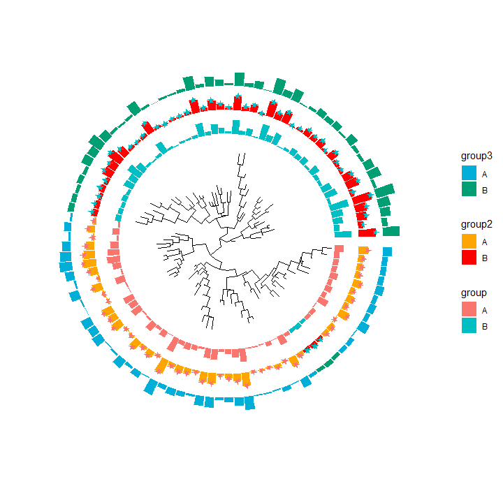
##随机树
# To reproduce.
set.seed(1024)
# generate 100 tip point tree.
tr <- rtree(100)
# I generate three datasets, which are the same except the third column name.
dt <- data.frame(id=tr$tip.label, value=abs(rnorm(100)), group=c(rep("A",50),rep("B",50)))
df <- dt
dtf <- dt
colnames(df)[[3]] <- "group2"
colnames(dtf)[[3]] <- "group3"
# plot tree
p <- ggtree(tr, layout="fan", open.angle=0)
#> Scale for 'y' is already present. Adding another scale for 'y', which will
#> replace the existing scale.
p

# the first ring.
p1 <- p +
  geom_fruit(
    data=dt,
    geom=geom_bar,
    mapping=aes(y=id, x=value, fill=group),
    orientation="y",
    stat="identity"
  ) +
  new_scale_fill()
p1
# the second ring
# geom_fruit_list is a list, which first element must be layer of geom_fruit.
p2 <- p1 +
  geom_fruit_list(
    geom_fruit(
      data = df,
      geom = geom_bar,
      mapping = aes(y=id, x=value, fill=group2),
      orientation = "y",
      stat = "identity"
    ),
    scale_fill_manual(values=c("orange", "red")), # To map group2
    new_scale_fill(), # To initialize fill scale.
    geom_fruit(
      data = dt,
      geom = geom_star,
      mapping = aes(y=id, x=value, fill=group),
      size = 2.5,
      color = NA,
      starstroke = 0
    )
  ) +
  new_scale_fill()
p2
# The third ring
p3 <- p2 +
  geom_fruit(
    data=dtf,
    geom=geom_bar,
    mapping = aes(y=id, x=value, fill=group3),
    orientation = "y",
    stat = "identity"
  ) +
  scale_fill_manual(values=c("#00AED7", "#009E73"))
p3

