验证方法:
1、训练集、线下验证集、线下测试集、线上测试集
2、无时序的数据集:简单划分、交叉验证划分等
3、有时序的数据集:需考虑时序,nested交叉验证划分等

目标函数:
与评价函数是不一样的,评价函数不会影像你的训练过程,但是目标函数会影像学习策略。
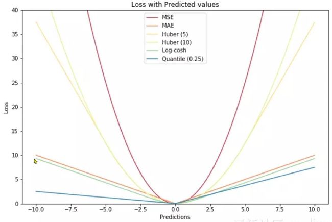
目标函数有很多种,有MAE、MSE、Huber(5)、Huber(10)、Log-cosh、Quantile(0.25)等。
本赛题的评价函数是MAE,但是MAE函数是分段函数,在loss=0处是不可导的,由于在训练模型的时候要计算梯度,不可导就不可计算梯度,所以使用其他函数来近似MAE,比如使用Huber函数。
最新版的LightGBM模型是预设了MAE函数的,对于效果的提升很好。
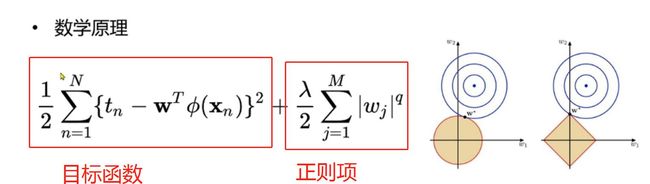
正则化:
奥卡姆剃刀原理:如无必要,毋增实体,那些比较不重要的特征,给小的权重。
数学原理:在目标函数后面,增加一个正则项,这样保证目标函数最小,正则项也最小。
机器学习就是求解一组最合适的,使损失最小。
加上正则项,就是要损失最小的同时,还要让绝对值的和(L1)或者平方的和(L2)最小。
做正则化之前要先做归一化。
代码实战
忽略warning警报
import warnings
warnings.filterwarnings('ignore')
读取特征
祖传降低内存代码,通过精度转换降低内存损耗。
def reduce_mem_usage(df):
    """ iterate through all the columns of a dataframe and modify the data type
        to reduce memory usage.
    """
    start_mem = df.memory_usage().sum()
    print('Memory usage of dataframe is {:.2f} MB'.format(start_mem))

    for col in df.columns:
        col_type = df[col].dtype

        if col_type != object:
            c_min = df[col].min()
            c_max = df[col].max()
            if str(col_type)[:3] == 'int':
                if c_min > np.iinfo(np.int8).min and c_max < np.iinfo(np.int8).max:
                    df[col] = df[col].astype(np.int8)
                elif c_min > np.iinfo(np.int16).min and c_max < np.iinfo(np.int16).max:
                    df[col] = df[col].astype(np.int16)
                elif c_min > np.iinfo(np.int32).min and c_max < np.iinfo(np.int32).max:
                    df[col] = df[col].astype(np.int32)
                elif c_min > np.iinfo(np.int64).min and c_max < np.iinfo(np.int64).max:
                    df[col] = df[col].astype(np.int64)
            else:
                if c_min > np.finfo(np.float16).min and c_max < np.finfo(np.float16).max:
                    df[col] = df[col].astype(np.float16)
                elif c_min > np.finfo(np.float32).min and c_max < np.finfo(np.float32).max:
                    df[col] = df[col].astype(np.float32)
                else:
                    df[col] = df[col].astype(np.float64)
        else:
            df[col] = df[col].astype('category')

    end_mem = df.memory_usage().sum()
    print('Memory usage after optimization is: {:.2f} MB'.format(end_mem))
    print('Decreased by {:.1f}%'.format(100 * (start_mem - end_mem) / start_mem))
    return df
sample_feature = reduce_mem_usage(pd.read_csv('data_for_tree.csv'))
选择连续特征做LR
continuous_feature_names = [x for x in sample_feature.columns if x not in ['price','brand','model']]
做个简单的特征工程
#删掉空值,替换“-”,重排index
sample_feature = sample_feature.dropna().replace('-', 0).reset_index(drop=True)
# astype更改数据类型
sample_feature['notRepairedDamage'] = sample_feature['notRepairedDamage'].astype(np.float32)
train = sample_feature[continuous_feature_names + ['price']]

train_X = train[continuous_feature_names]
train_y = train['price']
线性回归建模
from sklearn.linear_model import LinearRegression
model = LinearRegression(normalize=True)
model=model.fit(train_X,train_y)
查看训练的线性回归模型的截距(intercept)与权重(coef)
'intercept:'+ str(model.intercept_)
sorted(dict(zip(continuous_feature_names, model.coef_)).items(), key=lambda x:x[1], reverse=True)
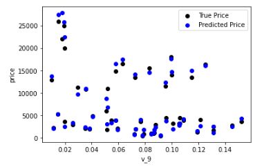
随机取出50个点,看看拟合效果
from matplotlib import pyplot as plt
subsample_index = np.random.randint(low=0,high=len(train_y),size=50)
plt.scatter(train_X['v_9'][subsample_index],train_y[subsample_index],color="black")
plt.scatter(train_X['v_9'][subsample_index],model.predict(train_X.loc[subsample_index]),color="blue")
plt.xlabel('v_9')
plt.ylabel('price')
plt.legend(['True Price','Predict Price'],loc="upper right")
print('The predict price is obvious different from true price')
plt.show()

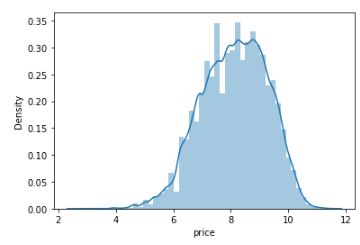
差异较大,而且预测出现负值。分析差异原因,发现标签的分布呈现长尾分布,要转化为正态。
考虑使用长尾截断,但是效果不明显。
import seaborn as sns
print("it is clear to see the price shows a typical exponential distribution")
plt.figure(figsize=(15,5))
plt.subplot(1,2,1)
sns.distplot(train_y)
plt.subplot(1,2,2)
sns.distplot(train_y[train_y
尝试使用log转换,这里log里面要+1,这样对于在0~1之间的特征x,不会变成一个很大的负数。如果x是负数,就平移一下再做log转换,也就是在log里面加更大的数。
train_y_ln=np.log(train_y+1)
sns.distplot(train_y_ln)
重新训练一下,看看效果如何
model= model.fit(train_X,train_y_ln)
print('intercept:'+ str(model.intercept_))
sorted(dict(zip(continuous_feature_names, model.coef_)).items(), key=lambda x:x[1], reverse=True)
plt.scatter(train_X['v_9'][subsample_index], train_y[subsample_index], color='black')
plt.scatter(train_X['v_9'][subsample_index], np.exp(model.predict(train_X.loc[subsample_index])), color='blue')
plt.xlabel('v_9')
plt.ylabel('price')
plt.legend(['True Price','Predicted Price'],loc='upper right')
print('The predicted price seems normal after np.log transforming')
plt.show()
五折交叉验证
from sklearn.model_selection import cross_val_score
from sklearn.metrics import mean_absolute_error,make_scorer
make_scorer是用于自定义评价函数。
这里下面再定义一个装饰器函数,用来装饰MAE计分函数,相当于把数据先进行一个log变换,然后再计算MAE的分值。
def log_transfer(func):
    def wrapper(y,yhat):
        result = func(np.log(y),np.nan_to_num(np.log(yhat)))
        return result
    return wrapper
scores = cross_val_score(model,X=train_X,y=train_y,verbose=1,cv=5,scoring=make_scorer(log_transfer(mean_absolute_error)))
print('AVG:',np.mean(scores))
这样做的原因,是因为这里想比较log转换前后,模型的拟合效果,评价方式是MAE,而log变换前后标签price的数量级是不一样的,故MAE的数量级也是不一样的。为了能比较二者差异,要将log变换前的数据也做一个log,再计算MAE。
对于已经做过log变换之后的数据,不需要再使用装饰器包装,直接计算MAE分值。
scores=cross_val_score(model,X=train_X,y=train_y_ln,verbose=1,cv=5,scoring=make_scorer(mean_absolute_error))
print('AVG:', np.mean(scores))
可将五折交叉验证的每个折的结果输出:
scores=pd.DataFrame(scores.reshape(1,-1))
scores.columns=['cv'+str(x) for x in range(1,6)]
scores.index=['MAE']
scores

时序数据的验证
由于我们并不具有预知未来的能力,五折交叉验证在某些与时间相关的数据集上反而反映了不真实的情况。通过2018年的二手车价格预测2017年的二手车价格,这显然是不合理的,因此我们还可以采用时间顺序对数据集进行分隔。在本例中,我们选用靠前时间的4/5样本当作训练集,靠后时间的1/5当作验证集,最终结果与五折交叉验证差距不大。
import datetime
sample_feature = sample_feature.reset_index(drop=True)
split_point = len(sample_feature) // 5 * 4

train = sample_feature.loc[:split_point].dropna()
val = sample_feature.loc[split_point:].dropna()

train_X = train[continuous_feature_names]
train_y_ln = np.log(train['price'] + 1)
val_X = val[continuous_feature_names]
val_y_ln = np.log(val['price'] + 1)

model = model.fit(train_X, train_y_ln)
mean_absolute_error(val_y_ln, model.predict(val_X))
# 输出结果0.195
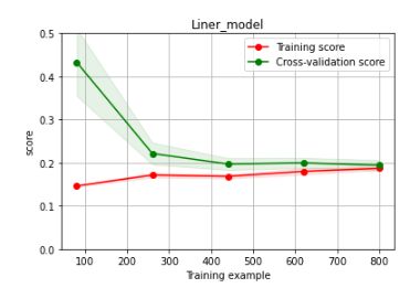
绘制学习率曲线与验证曲线
绘制曲线的函数代码可以直接复制使用。
from sklearn.model_selection import learning_curve, validation_curve
def plot_learning_curve(estimator, title, X, y, ylim=None, cv=None,n_jobs=1, train_size=np.linspace(.1, 1.0, 5 )):
    plt.figure()
    plt.title(title)
    if ylim is not None:
        plt.ylim(*ylim)
    plt.xlabel('Training example')
    plt.ylabel('score')
    train_sizes, train_scores, test_scores = learning_curve(estimator, X, y, cv=cv, n_jobs=n_jobs, train_sizes=train_size, scoring = make_scorer(mean_absolute_error))
    train_scores_mean = np.mean(train_scores, axis=1)
    train_scores_std = np.std(train_scores, axis=1)
    test_scores_mean = np.mean(test_scores, axis=1)
    test_scores_std = np.std(test_scores, axis=1)
    plt.grid()#区域
    plt.fill_between(train_sizes, train_scores_mean - train_scores_std,
                     train_scores_mean + train_scores_std, alpha=0.1,
                     color="r")
    plt.fill_between(train_sizes, test_scores_mean - test_scores_std,
                     test_scores_mean + test_scores_std, alpha=0.1,
                     color="g")
    plt.plot(train_sizes, train_scores_mean, 'o-', color='r',
             label="Training score")
    plt.plot(train_sizes, test_scores_mean,'o-',color="g",
             label="Cross-validation score")
    plt.legend(loc="best")
    return plt
plot_learning_curve(LinearRegression(), 'Liner_model', train_X[:1000], train_y_ln[:1000], ylim=(0.0, 0.5), cv=5, n_jobs=1)
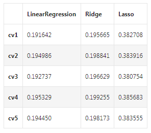
线性回归、岭回归、Lasso回归
嵌入式特征选择在学习器训练过程中自动地进行特征选择。嵌入式选择最常用的是L1正则化与L2正则化。
在对线性回归模型加入两种正则化方法后,他们分别变成了岭回归(L2)与Lasso回归(L1)。
train = sample_feature[continuous_feature_names + ['price']].dropna()
train_X=train[continuous_feature_names]
train_y=train['price']
train_y_ln=np.log(train_y)

from sklearn.linear_model import LinearRegression
from sklearn.linear_model import Ridge
from sklearn.linear_model import Lasso

models = [LinearRegression(),
         Ridge(),
         Lasso()]
分别使用三种回归模型进行交叉验证。
result = dict()
for model in models:
    model_name = str(model).split('(')[0]
    scores = cross_val_score(model,X=train_X,y=train_y_ln,verbose=0,cv=5,scoring=make_scorer(mean_absolute_error))
    result[model_name]=scores
    print(model_name+'is finished')
对三种方法的效果对比:
result = pd.DataFrame(result)
result.index = ['cv' + str(x) for x in range(1, 6)]
result
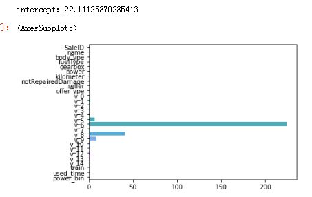
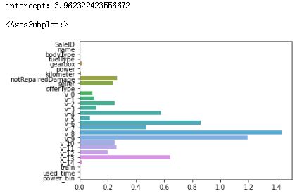
看一下LR回归模型的截距和系数:
model = LinearRegression().fit(train_X, train_y_ln)
print('intercept:'+ str(model.intercept_))
sns.barplot(abs(model.coef_), continuous_feature_names)
L2正则化(岭回归)在拟合过程中,通常都倾向于让权值尽可能小,最后构造一个所有参数都比较小的模型。一般认为权值比较小的模型比较简单,能适应不同的数据集,也在一定程度上避免了过拟合现象。可以设想一下对于一个线性模型,若参数很大,那么只要数据偏移一点点,就会对结果造成很大的影像,但是如果参数足够小,数据偏移得多一点也不会对结果造成什么影像,专业一点的说法,是“抗扰动能力强”。看一下岭回归(L2正则化)的截距和系数:
model = Ridge().fit(train_X,train_y_ln)
print('intercept:',str(model.intercept_))
sns.barplot(abs(model.coef_),continuous_feature_names)
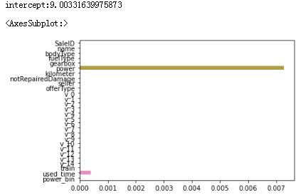
L1正则化(Lasso回归)有助于生成一个稀疏权值矩阵(很多特征的系数变成了0,相当于该特征被剔除了),进而可以用于特征选择。如下图,我们发现power与used_time非常重要。
model = Lasso().fit(train_X,train_y_ln)
print('intercept:'+str(model.intercept_))
sns.barplot(abs(model.coef_),continuous_feature_names)
除此之外,决策树通过信息熵或GINI指数选择分裂节点时,优先选择的分裂特征也更加重要,这同样是一种特征选择方法。XGBoost和LightGBM模型中的model_importance指标正是基于此计算的
非线性模型
除了线性模型之外,还有许多我们常用的非线性模型如下
from sklearn.linear_model import LinearRegression
from sklearn.svm import SVC
from sklearn.tree import DecisionTreeRegressor
from sklearn.ensemble import RandomForestRegressor
from sklearn.ensemble import GradientBoostingRegressor
from sklearn.neural_network import MLPRegressor
from xgboost.sklearn import XGBRegressor
from lightgbm.sklearn import LGBMRegressor
models = [
    LinearRegression(),
    DecisionTreeRegressor(),
    RandomForestRegressor(),
    GradientBoostingRegressor(),
    MLPRegressor(solver='lbfgs',max_iter=100),
    XGBRegressor(n_estimators = 100,objective="reg:squarederror"),
    LGBMRegressor(n_estimators=100)
]
result = dict()
for model in models:
    model_name = str(model).split('(')[0]
    scores = cross_val_score(model,X=train_X,y=train_y_ln,verbose=0,cv=5,scoring=make_scorer(mean_absolute_error))
    result[model_name]=scores
    print(model_name+"is finished")
result = pd.DataFrame(result)
result.index = ['cv' + str(x) for x in range(1, 6)]
result
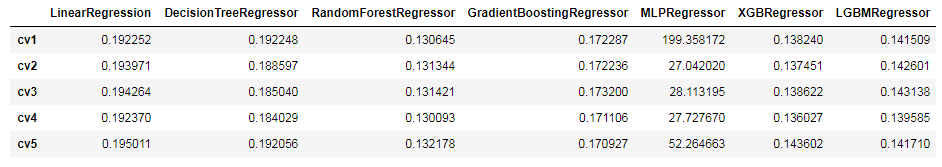
可以看到随机森林模型在每一个fold中均取得了更好的效果,但是根据经验,Lightgbm模型可以通过调参获得更大的提升。所以选择使用LGBM模型进行调参。
调参
贪心算法调参,一个参数调到最优,再调下一个。效果不如网格搜索,但是比网格搜索快。
贝叶斯调参的效率比网格搜索高很多,效果也比贪心算法好。可以了解一下。
## LGB的参数集合:
objective = ['regression','regression_l1','mape','huber','fair']
num_leaves = [3,5,10,15,20,40,55]
max_depth = [3,5,10,15,20,40,55]
bagging_fraction=[]
drop_rate=[]
贪心调参:
best_obj = dict()
for obj in objective:
    model = LGBMRegressor(objective=obj)
    score = np.mean(cross_val_score(model, X=train_X, y=train_y_ln, verbose=0, cv = 5, scoring=make_scorer(mean_absolute_error)))
    best_obj[obj] = score

best_leaves = dict()
for leaves in num_leaves:
    model = LGBMRegressor(objective=min(best_obj.items(), key=lambda x:x[1])[0], num_leaves=leaves)
    score = np.mean(cross_val_score(model, X=train_X, y=train_y_ln, verbose=0, cv = 5, scoring=make_scorer(mean_absolute_error)))
    best_leaves[leaves] = score

best_depth = dict()
for depth in max_depth:
    model = LGBMRegressor(objective=min(best_obj.items(), key=lambda x:x[1])[0],
                          num_leaves=min(best_leaves.items(), key=lambda x:x[1])[0],
                          max_depth=depth)
    score = np.mean(cross_val_score(model, X=train_X, y=train_y_ln, verbose=0, cv = 5, scoring=make_scorer(mean_absolute_error)))
    best_depth[depth] = score
sns.lineplot(x=['0_initial','1_turning_obj','2_turning_leaves','3_turning_depth'], y=[0.143 ,min(best_obj.values()), min(best_leaves.values()), min(best_depth.values())])

网格搜索调参
from sklearn.model_selection import GridSearchCV

parameters = {'objective': objective , 'num_leaves': num_leaves, 'max_depth': max_depth}
model = LGBMRegressor()
clf = GridSearchCV(model, parameters, cv=5)
clf = clf.fit(train_X, train_y)

clf.best_params_
model = LGBMRegressor(objective='regression',
                          num_leaves=55,
                          max_depth=15)

np.mean(cross_val_score(model, X=train_X, y=train_y_ln, verbose=0, cv = 5, scoring=make_scorer(mean_absolute_error)))
得到网格调参后的MAE分值是0.136。
贝叶斯调参
from bayes_opt import BayesianOptimization

def rf_cv(num_leaves, max_depth, subsample, min_child_samples):
    val = cross_val_score(
        LGBMRegressor(objective = 'regression_l1',
            num_leaves=int(num_leaves),
            max_depth=int(max_depth),
            subsample = subsample,
            min_child_samples = int(min_child_samples)
        ),
        X=train_X, y=train_y_ln, verbose=0, cv = 5, scoring=make_scorer(mean_absolute_error)
    ).mean()
    return 1 - val
rf_bo = BayesianOptimization(
    rf_cv,
    {
    'num_leaves': (2, 100),
    'max_depth': (2, 100),
    'subsample': (0.1, 1),
    'min_child_samples' : (2, 100)
    }
)
rf_bo.maximize()
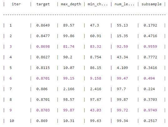
1 - rf_bo.max['target']
输出贝叶斯调参后的MAE分值约是0.129
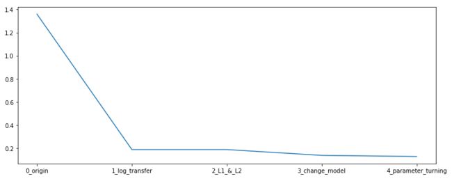
总结
在本章中,我们完成了建模与调参的工作,并对我们的模型进行了验证。此外,我们还采用了一些基本方法来提高预测的精度,提升如下图所示。
plt.figure(figsize=(13,5))
sns.lineplot(x=['0_origin','1_log_transfer','2_L1_&_L2','3_change_model','4_parameter_turning'], y=[1.36 ,0.19, 0.19, 0.14, 0.13])