数字图像处理(一)灰度变换与空间滤波(灰度变换,直方图处理,空间滤波,模糊处理)
灰度变换与空间滤波
- 1.1.背景知识
- 1.2.灰度变换函数
-
- 1.2.1.imadjust和stretchlim函数
-
- 1.2.1.1.以乳房图像为例展开研究
- 1.2.2.对数及对比度扩展变换
-
- 1.2.2.1.利用对数变换压缩动态范围
- 1.2.4.针对灰度变换的函数
-
- 1.2.4.1.处理数目可变的函数的输入
- 1.2.4.2.tofloat函数
- 1.2.4.3.intrans函数
- 1.2.4.2.例子展示
- 1.3.直方图处理与函数绘图综述
-
- 1.3.1.生成并绘制图像的直方图
-
- 1.3.1.2.imhist(),bar(),stem(),plot()绘图函数综述:
- 1.3.1.3.举例说明:
- 1.3.2.直方图均衡化
-
- 1.3.2.1.概述:
- 1.3.2.2.代码实现及举例说明:
- 1.3.3.直方图匹配化(规定化)
-
- 1.3.3.1.概述:
- 1.3.3.2.工具箱函数:
- 1.3.3.3.举例说明:
- 1.3.4.函数adapthisteq
- 1.4.空间滤波
-
- 1.4.1.线性空间滤波
-
- 1.4.1.1.原理介绍
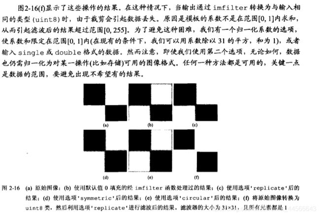
- 1.4.1.2.imfilter函数介绍
- 1.4.2.非线性空间滤波
-
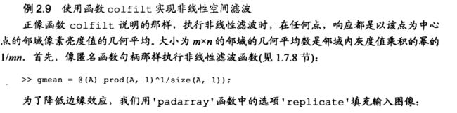
- 1.4.2.1.理论概述
- 1.4.2.2.工具箱函数
- 1.4.2.3.举例说明
- 1.5.图像处理工具箱中的标准空间滤波器
-
- 1.5.1.线性空间滤波器
- 1.5.1.1.工具箱函数概述
-
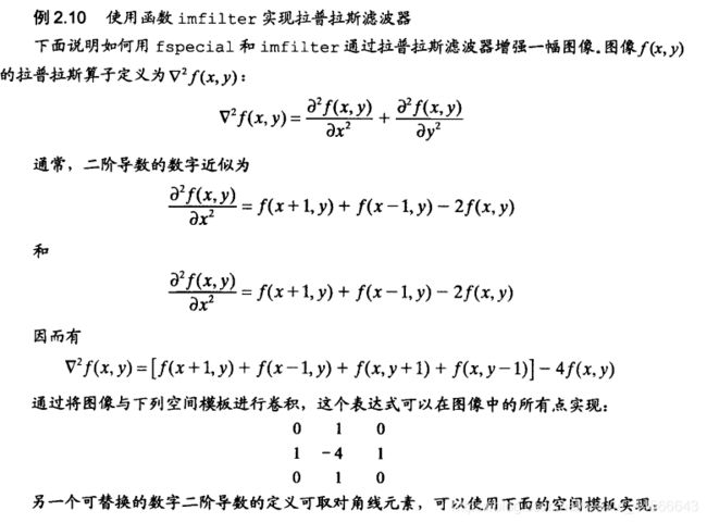
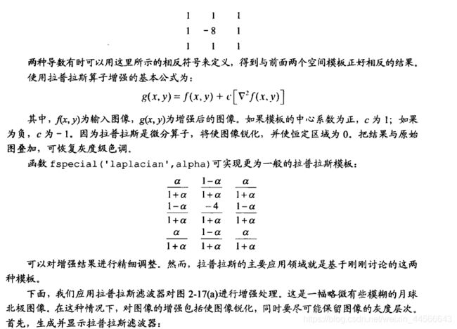
- 1.5.1.2.使用函数imfilter实现拉普拉斯算子
- 1.5.1.3.八邻域拉普拉斯图像
- 1.5.2.非线性空间滤波器
- 1.5.2.1.基本概念:
- 1.5.2.2.例题展示(中值滤波)
- 1.6.将模糊技术用于灰度变换和空间滤波
-
- 1.6.1.背景知识
- 1.6.2.将模糊集合用于灰度变换
- 1.6.6.将模糊集合用于空间滤波
- 1.7.小结
1.1.背景知识
(1)空间域:指的是图像平面本身,这类方法以对图像进行直接处理为基础;
(2)两种重要的空间域处理方法灰度变换与空间滤波;
为了保持主题的一致性,我们本章大部分示例都和图像增强相关。
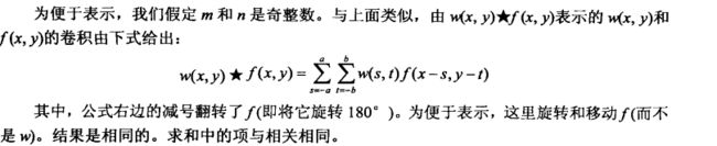
前面已经指出,空间域技术直接对图像的像素进行操作。本章中讨论的空间域处理由下列表达式表示:

1.2.灰度变换函数
变换的最简单形式就是上图中邻域大小为1x1,单个像素的情况,T就是灰度变换函数
由于输出值仅取决于点的灰度值,而不是取决于点的邻域,因此灰度变换函数通常写成如 下简单形式: 
1.2.1.imadjust和stretchlim函数
imadjust 函数是针对灰度图像进行灰度变换的基本图像处理工具箱函数,一般的语法格 式如下:g = imadjust(f,[low_in high_in],[low_out high_out],gamma)

1.2.1.1.以乳房图像为例展开研究


%%读取原始图像
f=imread('Fig0203(a).tif');
%%显示负片图像,0变成1,1变成0
%%注意此操作也可以通过imcomplement函数来得到
g1=imadjust(f,[0 1],[1 0]);
%%将0.5到0.75的亮度范围扩展到0到1整个范围,强调一下感兴趣的灰度区域
g2=imadjust(f,[0.5 0.75],[0 1]);
%%指定gamma>2,但并不强调是哪一片灰度区域,不用再自己去设置高低参数
g3=imadjust(f,[],[],2);
%%实际上stretch函数可以胜任这个工作,
Low_High=stretchlim(f);
g4=imadjust(f,stretchlim(f),[]);
%%再来尝试生成负片图像,该操作可以增强负片的对比度
g5=imadjust(f,stretchlim(f),[1 0]);
%%绘图
figure
subplot(231);imshow(f);title('原始数字乳房图像');
subplot(232);imshow(g1);title('负片图像');
subplot(233);imshow(g2);title('[0.5 0.75]扩至[0 1]的结果');
subplot(234);imshow(g3);title('gamma=2增强后的结果');
subplot(235);imshow(g4);title('对原始图像使用stretchlim函数对比度增强');
subplot(236);imshow(g5);title('stretchlim函数也增强负片图像的对比度');

1.2.2.对数及对比度扩展变换
对数及对比度扩展变换是动态范围处理的基本工具。对数变换通过下列表达式实现:

对数变换的一项主要应用是压缩动态范围。例如,傅立叶频谱(参见第 3 章)的范围在[0,106; 1 或更高范围是常见的,当监视器显示范围线性地显示为 8 位时,高值部分较占优势,从而导致 频谱中低灰度值的细节部分丢失
在执行对数变换的时候,通常期望的是将压缩值返回到显示的全域
以uint8图像为例:

1.2.2.1.利用对数变换压缩动态范围


clear;
g=imread('Fig0205(a).tif');
g1=im2uint8(mat2gray(log(1+double(g))));
figure
subplot(121);imshow(g);title('原始傅里叶频谱');
subplot(122);imshow(g1);title('使用对数变换后的结果');0
1.2.4.针对灰度变换的函数
1.2.4.1.处理数目可变的函数的输入
为检测输入到函数的参量的数目,我们利用nargin函数
n=nargin%%可以返回输入到函数的参量的实际数量
n=nargout%%与之相似,可用于输出
1.2.4.2.tofloat函数
这个是工具箱中附加的自定义函数,
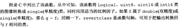
再用到的时候不妨查函数表
1.2.4.3.intrans函数
这个我们开发的函数可以执行下列变换:负片变换,对数变换,gamma变换以及对比度扩展
(1)代码研读
function g = intrans(f, varargin)
%内部函数执行强度(灰度级)转换。
% G = INTRANS(F, 'neg') 计算输入图像F的负数。
%
% G = INTRANS(F, 'log', C, CLASS)计算C*log(1 + F)和
%将结果乘以(正的)常数c,如果最后两个参数省略,C默认为1。因为使用了对数
%经常显示傅里叶谱,参数类提供了
%选项将输出的类指定为'uint8'或
%的“uint16”。如果省略参数类,则输出为与输入相同的类。
%
% G = INTRANS(F, 'gamma', GAM) 执行伽马变换
%使用参数GAM(一个必需的输入)输入图像。
%
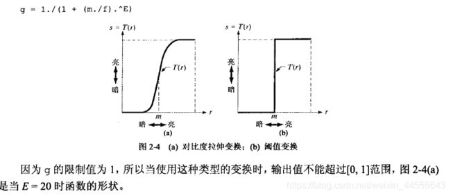
% G = INTRANS(F, 'stretch', M, E) 计算一个对数扩展 1./(1 + (M./(F +
% eps)).^E). 参数M必须限制在 [0, 1]. 默认的M的值为
%mean2(im2double(F)), E的默认值为是4。
%
% 对于 'neg', 'gamma', and 'stretch' 变换, double
% input images 最大值大于1的先用 MAT2GRAY进行缩放. 其他图像先转换成double
% 用IM2DOUBLE. 对于 'log'变换, double images are
% transformed without being scaled; 其他图像先用 IM2DOUBLE转换成double.
%
% 输出与输入属于同一类,除非a为“log”选项指定了%不同的类。
% 验证输入的正确数量。
error(nargchk(2, 4, nargin))
% 存储输入的类以供以后使用。
classin = class(f);
% 如果输入的类是double, 并且超出了范围
% [0, 1], 并且指定的转换不是 'log', 则转换输入到范围【0 1】
if strcmp(class(f), 'double') & max(f(:)) > 1 & ...
~strcmp(varargin{
1}, 'log')
f = mat2gray(f);
else % 转换成double, 无视class(f).
f = im2double(f);
end
% 确定指定的转换类型
method = varargin{
1};
% 执行指定的灰度转换。
switch method
case 'neg'
g = imcomplement(f);
case 'log'
if length(varargin) == 1
c = 1;
elseif length(varargin) == 2
c = varargin{
2};
elseif length(varargin) == 3
c = varargin{
2};
classin = varargin{
3};
else
error('Incorrect number of inputs for the log option.')
end
g = c*(log(1 + double(f)));
case 'gamma'
if length(varargin) < 2
error('Not enough inputs for the gamma option.')
end
gam = varargin{
2};
g = imadjust(f, [ ], [ ], gam);
case 'stretch'
if length(varargin) == 1
% 使用默认值
m = mean2(f);
E = 4.0;
elseif length(varargin) == 3
m = varargin{
2};
E = varargin{
3};
else error('Incorrect number of inputs for the stretch option.')
end
g = 1./(1 + (m./(f + eps)).^E);
otherwise
error('Unknown enhancement method.')
end
% 转换为输入图像的类。
g = changeclass(classin, g);
1.2.4.2.例子展示

clear;
f=imread('Fig0206(a).tif');
g=intrans(f,'stretch',mean2(tofloat(f)),0.9);
figure
subplot(121);imshow(f);title('骨骼扫描原始图像');
subplot(122);imshow(g);title('对比度扩展变换增强后的图像');
1.3.直方图处理与函数绘图综述
以从图像灰度直方图中提取信息为基础的灰度变换函数在诸如增强、压缩、分割、描述等 方面的图像处理中起重要作用。本节的重点放在获取、绘图并利用直方图技术进行图像增强方 面
1.3.1.生成并绘制图像的直方图

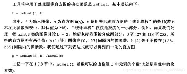
1.3.1.2.imhist(),bar(),stem(),plot()绘图函数综述:


1.3.1.3.举例说明:
以前面的原始乳房图像为例说明:

clc;
clear;
%%读取原始乳房图像
f=imread('Fig0203(a).tif');
%%屏幕绘制直方图的最简便方法,利用没有输出规定的imhist函数
figure
subplot(221);imhist(f);title('经典直方图');
%%也可以用条形图来绘制直方图
h=imhist(f,25);
horz = linspace(0, 255, 25);%%0到255分成25分
subplot(222);bar(horz, h) ;%%注意维度必须相同
axis([0 255 0 60000]);
set(gca, 'xtick', 0:50:255);
set(gca, 'ytick', 0:20000:60000);
title('条形图')
%%使用杆状图绘制直方图
horz = linspace(0, 255, 25);
subplot(223);title('杆状图');
stem(horz, h, 'fill');
axis([0 255 0 60000]);
set(gca, 'xtick', [0:50:255]);
set(gca, 'ytick', [0:20000:60000]);
%%使用plot函数绘制
 he = imhist(f);
 subplot(224);
 plot(he); % Use the default values.
 title('plot绘图');
 axis([0 255 0 15000]) ;
 set(gca, 'xtick',[0:50:255]);
 set(gca, 'ytick',[0:2000:15000]);
1.3.2.直方图均衡化
1.3.2.1.概述:


1.3.2.2.代码实现及举例说明:

举例说明:


clc;
clear;
f=imread('Fig0208(a).tif');
figure;
subplot(221);imshow(f);title('原始花粉图像');
subplot(222);imhist(f);ylim('auto');title('原始图像对应的直方图');
g=histeq(f,256);
subplot(223);imshow(g);title('直方图均衡化之后的图像');
subplot(224);imhist(g);ylim('auto');title('直方图均衡化之后的直方图');
1.3.3.直方图匹配化(规定化)
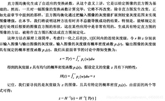
1.3.3.1.概述:
生成具有规定直方图的图像的方法:

1.3.3.2.工具箱函数:

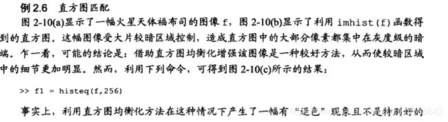
1.3.3.3.举例说明:

clc;
clear;
f=imread('Fig0210(a).tif');
figure
subplot(221);imshow(f);title('原始天体图像');
subplot(222);imhist(f);ylim('auto');title('原始天体图像对应的直方图');
g=histeq(f,256);
subplot(223);imshow(g);title('直方图均衡化后的图像');
subplot(224);imhist(g);title('均衡化后的土相对应的直方图');


clc;
clear;
f=imread('Fig0210(a).tif');
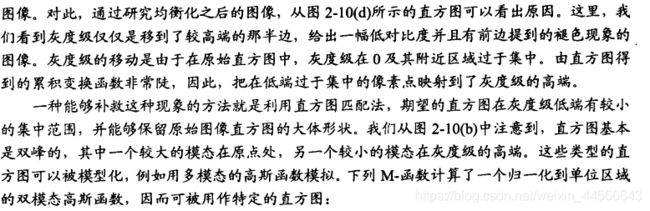
p=twomodegauss(0.15,0.05,0.75,0.05,1,0.07,0.002);%%双模高斯常常这么设置
figure
g=histeq(f,p);
subplot(2,2,[1 3]);imhist(g);title('规定化后的对应的直方图');
subplot(222);plot(p);
title('plot绘图');
subplot(224);imshow(g);title('直方图规定化后的图像');
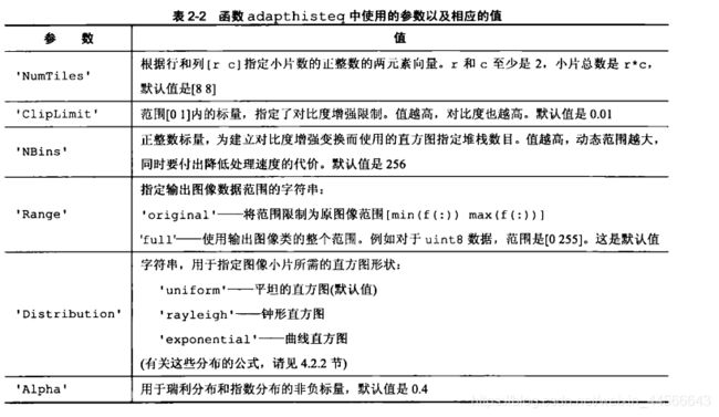
1.3.4.函数adapthisteq
此工具箱函数执行所谓的对比度受限的自适应直方图均衡化,这个方法是由用直方图规定化方法处理图像的小区域(称为小片组成),之后用双线性内插将相邻小片组合起来以消除人工引入的边界效应

举例说明


clc;
clear;
f=imread('Fig0210(a).tif');
g1=adapthisteq(f);
g2=adapthisteq(f,'NumTiles',[25 25]);
g3=adapthisteq(f,'NumTiles',[25 25],'ClipLimit',0.05);
figure
subplot(221);imshow(f);title('原始图像');
subplot(222);imshow(g1);title('用adapthisteq函数并默认值');
subplot(223);imshow(g2);title('用adapthisteq函数并指定小片数为25x25');
subplot(224);imshow(g3);title('用adapthisteq函数并指定对比度')
1.4.空间滤波

![]()
1.4.1.线性空间滤波
1.4.1.1.原理介绍


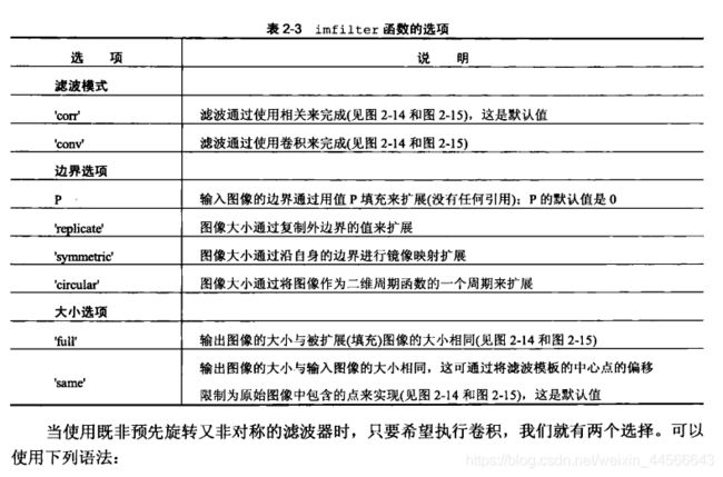
1.4.1.2.imfilter函数介绍
(1)函数说明


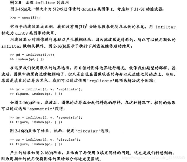
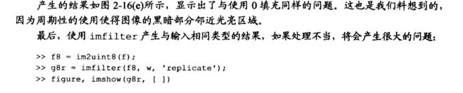
(2)函数应用举例
1.4.2.非线性空间滤波
1.4.2.1.理论概述

1.4.2.2.工具箱函数


1.4.2.3.举例说明

1.5.图像处理工具箱中的标准空间滤波器
这一节我们使用工具箱函数来实现线性空间滤波与非线性空间滤波
1.5.1.线性空间滤波器
1.5.1.1.工具箱函数概述


1.5.1.2.使用函数imfilter实现拉普拉斯算子

1.5.1.3.八邻域拉普拉斯图像
(1)运行结果展示:

(2)代码展示:
clc;
clear;
f=imread('Fig0217(a).tif');
w=fspecial('laplacian',0);%实际上在这个地方我们就是调用一下生成一个参数矩阵,
%牵扯到类型转换,直接据此写出该参数矩阵
w=[0 1 0;1 -4 1;0 1 0];
figure
subplot(221);imshow(f,[]);title('原始月球北极图像');
g1=imfilter(f,w,'replicate');
subplot(222);imshow(g1,[]);title('使用uint8格式的拉普拉斯滤波后图像');
f2=tofloat(f);
g2=imfilter(f2,w,'replicate');
subplot(223);imshow(g2,[]);title('使用浮点格式的拉普拉斯滤波后的图像')
g=f2-g2;
subplot(224);imshow(g);title('增强后的结果,a-c');


(1)运行结果展示:

clc;
clear;
f=imread('Fig0217(a).tif');
w4=fspecial('laplacian',0);%像上一个例子一样
w8=[1 1 1;1 -8 1;1 1 1];
f=tofloat(f);
g4=f-imfilter(f,w4,'replicate');
g8=f-imfilter(f,w8,'replicate');
figure
subplot(221);imshow(f);title('原始图像');
subplot(222);imshow(g4);title('4邻域拉普拉斯增强后的图像');
subplot(223);imshow(g8);title('8邻域拉普拉斯增强后的图像');
1.5.2.非线性空间滤波器
1.5.2.1.基本概念:


1.5.2.2.例题展示(中值滤波)

(1)结果展示:

(2)代码概述
clc;
clear;
f=imread('Fig0219(a).tif');
fn=imnoise(f,'salt & pepper',0.2);
gm=medfilt2(fn);
gms=medfilt2(fn,'symmetric');
figure
subplot(221);imshow(f);title('原始X射线图像');
subplot(222);imshow(fn);title('由椒盐噪声污染的图像');
subplot(223);imshow(gm);title('用函数medfilt2默认处理的结果');
subplot(224);imshow(gms);title('加上选项symmetric处理,边缘效应改进');
1.6.将模糊技术用于灰度变换和空间滤波
简要介绍模糊集合及其在灰度变换及空间滤波方面的应用
1.6.1.背景知识

此部分内容较多,我们在后续用到了可以详细研究,此处不做赘述
1.6.2.将模糊集合用于灰度变换
(1)用模糊函数实现对比度增强

1.6.6.将模糊集合用于空间滤波

1.7.小结
这一章的内容是处理后续众多话题的基础,我们会在噪声消除,边缘检测,空间滤波等众多方面展开讨论,