DeepLearning——模型压缩剪枝量化
-
模型压缩
-
为什么需要模型压缩
-
量化
-
剪枝
-
蒸馏
模型压缩
为什么需要模型压缩
- 深度学习(Deep Learning)因其计算复杂度或者参数冗余,在一些场景和设备上限制了相应的模型部署,因此需要模型压缩、优化加速、异构计算等方法突破瓶颈。
- 其实我们一般用框架训练好了模型的权重之后,我们需要把模型安装到其他设备上,例如PC端、服务器、嵌入式板子树莓派、tensorRT等等,不是所有的设备都具有我们训练时候的那种推理和计算能力。像嵌入式板子那种,对性能和功耗都有严格要求的,你总不能强迫公鸡下蛋吧。这样模型压缩算法的提出就应运而生啦。
- 模型压缩算法能够有效的降低参数冗余,从而减少存储占用、通信宽带和计算复杂度,有助于深度学习的应用部署。具体可以划分为如下几种方法(后续重点介绍剪枝和量化):
| 总结 | 方法 |
|---|---|
| 线性或者非线性量化 | 1/2bits,int8和fp16等 |
| 结构或非结构剪枝 | deep compression,channel pruning和network slimming等 |
| 网络结构搜索 | NAS:Network Architecture Search:DARTS,DetNAS和NAS-FCOS |
| 权重矩阵的低秩分解 | 知识蒸馏与网络结构简化(Squeeze-net,mobile-net,shuffle-net) |
剪枝
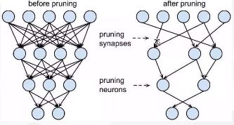
- ☆剪枝时,针对净输出进行L1正则化,对净输出进行归一化约束,然后对净输出进行L1正则化,这样在把不必要权重剪枝的情况下,可以加大需要的权重,能力转移。
- 工业运作是经常剪得就是神经元,如果剪神经元的参数,尽管参数变为0没有作用,但是在网络模型计算时仍然会进入模型计算。基本在支持精细化计算的时候才会使用参数剪枝。剪神经元则会相对应的减少计算量。
卷积核的剪枝

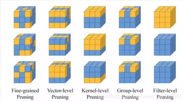
| 剪枝方法 | 依据 |
|---|---|
| 随机裁剪 | 随机 |
| 裁剪向量 | 计算二范数大小 |
| 裁剪核 | 对核进行裁剪 |
| 裁剪组 | 针对固定组的剪 |
| 裁剪通道 | 正常情况下用这个 |

- 剪枝常用手段
| 方法 | 描述 |
|---|---|
| 非结构剪枝 | 通常是连接级、细粒度的剪枝方法、精度相对较高,但是依赖于特定的算法库或者硬件平台的支持,如Deep Compression,Sparse-Winograd |
| 结构剪枝 | filter级或者layer级、粗粒度的剪枝方法,精度相对降低,但是剪枝策略更为有效,不需要特定算法库或者硬件平台的支持,能够直接在成熟深度学习框架上运行 |
结构剪枝
- 局部方式,通过layer by layer方式,最小化输出FM重建误差的Channel Pruning,ThiNet ,Discrimination-aware Channel Pruning。
- 全局方式的、通过训练期间对BN层Gamma系数添加L1正则化的Network Slimming;
- 全局方式的、按Taylor准则对Filter做重要性排序的Neuron Pruning;
- 全局方式的、可动态更新更新pruned filters 参数的剪枝方法;
- 基于GAN思想的GAL方法,可裁剪包括Channel,Branch或Block等在内的异构结构;
- 借助Geometric Median确定卷积滤波器冗余性的剪枝策略;
- 基于Reingorcement Learning(RL) 实现每一层剪枝率的连续、精细控制,并可结合资源约束完成自动模型压缩;
SeNet网络权重剪枝思想
- 卷积核,为了判断卷积核中那些比较有用,可以让卷积核乘以一个标量w形成一个新的卷积核,在反向梯度更新时,观察w的大小,可以知道每个卷积核的重要性比重权重,这样就可以知道哪些卷积核重要性。
代码演示
局部剪枝
import torch
from torch import nn
import torch.nn.utils.prune as prune
import torch.nn.functional as F

device = torch.device("cuda" if torch.cuda.is_available() else "cpu")

class LeNet(nn.Module):
    def __init__(self):
        super(LeNet, self).__init__()
        # 1 input image channel, 6 output channels, 3x3 square conv kernel
        self.conv1 = nn.Conv2d(1, 6, 3)
        self.conv2 = nn.Conv2d(6, 16, 3)
        self.fc1 = nn.Linear(16 * 5 * 5, 120)  # 5x5 image dimension
        self.fc2 = nn.Linear(120, 84)
        self.fc3 = nn.Linear(84, 10)

    def forward(self, x):
        # 最大赤化
        x = F.max_pool2d(F.relu(self.conv1(x)), (2, 2))
        x = F.max_pool2d(F.relu(self.conv2(x)), 2)
        x = x.view(-1, int(x.nelement() / x.shape[0]))
        x = F.relu(self.fc1(x))
        x = F.relu(self.fc2(x))
        x = self.fc3(x)
        return x
model = LeNet().to(device=device)
按照pytorch上的代码先定义了一个网络结构,按照下一步代码main函数运行可以得到得到对应结果。
	# 定义模型一个卷积层
    module = model.conv1
    # 打印该层模型的参数
    print(list(module.named_parameters()))
可以看到这一层的weight和bias
	# 用于剪枝时临时缓存的一些数据
	print(list(module.named_buffers()))
结果:[]
'''要修剪模块(conv1LeNet体系结构的层),请首先从中可用的修剪技术中选择修剪技术torch.nn.utils.prune(或 通过子类实现您自己 的修剪技术 BasePruningMethod)。然后,指定模块以及该模块中要修剪的参数的名称。最后,使用所选修剪技术所需的适当关键字参数,指定修剪参数。'''
	from torch.nn.utils import prune
	# 随机剪枝方法,针对这个模型的weight进行剪枝,剪枝比例0.3
	prune.random_unstructured(module, name="weight", amount=0.3)
下列运行代码:
# 函数运行
if __name__ == '__main__':
model = LeNet().to(device=device)
# 获取卷积层
module = model.conv1
# 打印参数,包括weight和偏值bias
print(list(module.named_parameters()))
# 剪枝时临时更改存储的数据掩码
print(list(module.named_buffers()))
# 按照0.3的权重比例,对网络该层的weight随机裁剪
prune.random_unstructured(module, name="weight", amount=0.3)
# 查看变化,看着值还没更改,但是已经生成了更改掩码,weight--->weight_orig(即追加"_orig"到初始参数name)来进行的。weight_orig存储未经修剪的张量版本。
# print(list(module.named_parameters()))
# 通过上面选择的修剪技术生成的修剪掩码被保存为名为weight_mask(即附加"_mask"到初始参数name)的模块缓冲区。
# print(list(module.named_buffers()))
# 已经改了
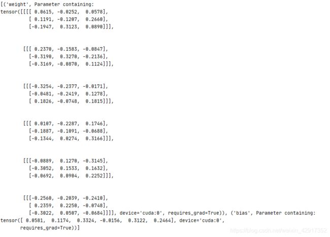
print(module.weight)
# 只显示对weight出现操作
print(module._forward_pre_hooks)
# L1剪枝。针对bias,剪3个最小的
prune.l1_unstructured(module, name="bias", amount=3)
# 打印,现在已经改为weight_orig 和 bias_orig
print(list(module.named_parameters()))
print(list(module.named_buffers()))
print(module._forward_pre_hooks)
- 剪枝尽量针对输出剪枝,针对输入剪枝不易操作。
 # 迭代修剪
    model = LeNet().to(device=device)
    # 获取卷积层
    module = model.conv1
    # dim :针对输出还是输入去剪枝,具体看形状 n:1,2 表示是L1,还是L2剪枝 name:针对weight还是bias
    prune.ln_structured(module, name="weight", amount=0.5, n=2, dim=0)
    print(module.weight)
    # 所有相关的张量,包括掩码缓冲区和用于计算修剪张量的原始参数,都存储在模型中state_dict ,因此可以根据需要轻松地序列化和保存。
    print(model.state_dict().keys())
    # 修剪永久化
    prune.remove(module, 'weight')
- 多参数剪枝
for name, module in new_model.named_modules():
    # prune 20% of connections in all 2D-conv layers
    if isinstance(module, torch.nn.Conv2d):
        prune.l1_unstructured(module, name='weight', amount=0.2)
    # prune 40% of connections in all linear layers
    elif isinstance(module, torch.nn.Linear):
        prune.l1_unstructured(module, name='weight', amount=0.4)

print(dict(new_model.named_buffers()).keys())  # to verify that all masks exist
全局剪枝
model = LeNet()

parameters_to_prune = (
    (model.conv1, 'weight'),
    (model.conv2, 'weight'),
    (model.fc1, 'weight'),
    (model.fc2, 'weight'),
    (model.fc3, 'weight'),
)

prune.global_unstructured(
    parameters_to_prune,
    pruning_method=prune.L1Unstructured,
    amount=0.2,
   ''' 我们可以检查在每个修剪参数中引起的稀疏度,该稀疏度将不等于每层中的20%。但是,全局稀疏度将(大约)为20%。'''
)
量化
- 低精度(Low precision)可能是最通用的概念。常规精度一般使用FP32(单精度32位浮点数)存储模型权重;低精度则表示FP16(半精度16位),INT8(8位的定点整数)等等数值格式,目前低精度往往指代INT8。
- 混合精度(Mixed precision)在精度中使用FP32和FP16。FP16减少了一般的内存大小,但有些参数或者操作符必须采用FP32的格式才可以保持准确度。
- 量化一般指INT8,将FP32类型转换为INT8类型,在损失少量精度的情况下,我们可以获得接近四倍的网络模型加速。
- 为了解决存储和带宽的开销需求,获得更低的能耗和占用面积,同时获得更快的计算速度
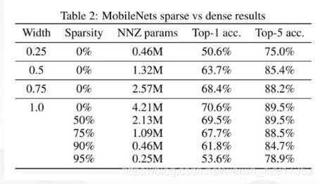
- 尚可接受的精度损失。即量化相当于对模型权重引入噪声,所幸CNN本身对噪声不敏感(在模型训练过程中,模拟量化所引入的权重加噪还有利于防止过拟合),在合适的比特数下量化后的模型并不会带来很严重的精度损失。按照gluoncv提供的报告,经过int8量化之后,ResNet50_v1和MobileNet1.0 _v1在ILSVRC2012数据集上的准确率仅分别从77.36%、73.28%下降为76.86%、72.85%。
- 根据存储一个权重元素所需要的的位数还可以有以下的方法:
| 神经网络 | 方法 |
|---|---|
| 二值神经网络 | 在运行时权重和激活只取两种值(例如+1,-1)的神经网络,以及在训练师计算参数的梯度 |
| 三元权重网络 | 权重约束为+1,0,-1的神经网络 |
| XNOR网络 | 过滤器和卷积层的输入是二进制的。XNOR网络主要视同二进制运算来近似卷积 |
- 理论是一回事,实践又是一回事,如果一种技术方法难以推广到通用场景,泽需要进行大量的额外支持。花里胡哨的研究往往是过于棘手或前提假设过于强,以至于无法引入工业界。
- 工业界最终选择是INT8量化——FP32在推理(inference)期间被INT8取代,训练仍然是FP32。TensorRT,TensorFlow,PyTorch.MxNet和其他许多深度学习软件都已经启用(或正在启用)量化。
- 通常可以根据FP32和INT8的转换机制来对解决方案进行分类。一些框架简单地引入了Quantize和Dequantize层,当从卷积或全链接层送入或者取出时,它将FP32转换为INT8或相反。在这种情况下,模型本身的输入/输出采用FP32格式。深度学习框架加载模型,重写网络以插入Quantize和Dequantize层,并且将权重转换为INT8格式。

- 在上图越往边上,下方映射的区间就代表更宽的区间,由于神经网络训练出来的权重一般都在0附近,那么在0附近可以近似于等分。
方法一:

方法2:

- 静态量化
- 尽量 让卷积、BN、Relu组成结构
- 按照pytorch官网实现量化简单例子
- 对原始的网络结构调整
- 在前向计算时量化,后向反量化
蒸馏
- 原理
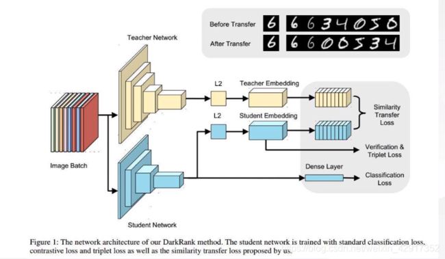
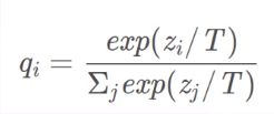
- 用能量温度的角度来看的话,初始温度设置高,模型会变得活跃,这样把老师模型(大模型)变得活跃,大模型学习硬标签,小模型跟着大模型一起学习,不过小模型学习的是大模型的输出,学习软标签。这样不断将温度调低,大模型就会渐渐变得稳定下来,也就是学习难度慢慢增大。小模型根据之前的软标签学习已经学习到一定经验,尽管学习难度增大,但是由于经验的原因,仍然可以继续学习。
蒸馏法升级(fps)


在特征层加上l2正则化损失,从特征层就开始学习,最后总损失是损失+特征层损失。
(NAS)
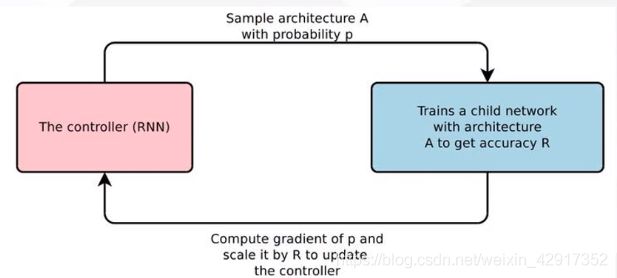
- 神经架构生成,自动搜索
- 废钱——不想做
模拟退火法
- paddleSlim(轻量级的集成框架,效果试过,不怎么好)

- 也有蒸馏思想,不断对小模型进行扰动,还加入了一定的探索机制。
- 反正自己找的就是慢TT(平民玩家不好玩)
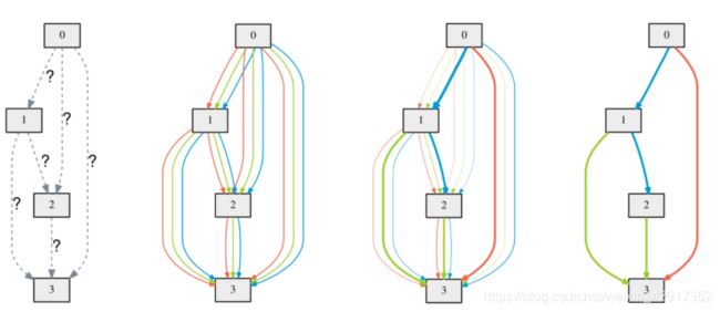
可微分神经架构搜索
- 最近的研究——基于梯度的架构搜索(DARTS)
- 先定义几个初始结构,卷积,最大池化等等,
- 然后后面的结构全部与前面结构相连
- 在每种结构前加一个系数w,开始训练,最后做一个softmax,就可以得到概率最大的那条线的组件。哪一个权重最大留哪条线(有点类似动态剪枝)