参考学习资料:https://academic.oup.com/bioinformatics/article/34/14/2515/4917355
之前看了技能树的系列推文和曾老师的推荐的文献,对ce-RNA有了初步的认识,为这个教程的理解奠定了理论基础。
1 安装包GDCRNATools及相关依赖包
rm(list = ls())
options(stringsAsFactors = F)
#if (!requireNamespace("BiocManager", quietly=TRUE)) install.packages("BiocManager")
#BiocManager::install("GDCRNATools", version = "devel")这个版本的需要R版本'4.0'
## try http:// if https:// URLs are not supported if (!requireNamespace("BiocManager", quietly=TRUE))
BiocManager::install("GDCRNATools")
BiocManager::install("DT")
library(GDCRNATools)
library(DT)
2 准备测试数据
在GDCRNATools中有些函数被设计来帮助其他人有效的下载和处理GDC数据。当然用户也可以用他们自己的数据从UCSC Xena GDC hub, TCGAbiolinks(Colaprico et al. 2016)等处获取的,或者TCGA-Assembler(Zhu, Qiu, and Ji 2014)都可以。
具体见case study
library(DT)
### load RNA counts data
data(rnaCounts)
### load miRNAs counts data data(mirCounts)
data(mirCounts)
2.1Normalization of HTSeq-Counts data
####### Normalization of RNAseq data #######
rnaExpr <- gdcVoomNormalization(counts = rnaCounts, filter = FALSE)
####### Normalization of miRNAs data #######
mirExpr <- gdcVoomNormalization(counts = mirCounts, filter = FALSE)
2.2 Parse metadata
####### Parse and filter RNAseq metadata #######
metaMatrix.RNA <- gdcParseMetadata(project.id = 'TCGA-CHOL',
                                   data.type  = 'RNAseq',
                                  write.meta = FALSE)
metaMatrix.RNA <- gdcFilterDuplicate(metaMatrix.RNA)
metaMatrix.RNA <- gdcFilterSampleType(metaMatrix.RNA)
datatable(as.data.frame(metaMatrix.RNA[1:5,]), extensions =
            'Scroller',options = list(scrollX = TRUE, deferRender = TRUE,
                                      scroller = TRUE))
样本信息输出列表:

3 ceRNAs network analysis
3.1 Identication of dierentially expressed genes (DEGs)
DEGAll <- gdcDEAnalysis(counts = rnaCounts,
                        group = metaMatrix.RNA$sample_type,
                        comparison = 'PrimaryTumor-SolidTissueNormal',
                        method = 'limma')
datatable(as.data.frame(DEGAll),
          options = list(scrollX = TRUE, pageLength = 5))
差异基因列表:

所有差异基因分类获取
### All DEGs
deALL <- gdcDEReport(deg = DEGAll, gene.type = 'all')
### DE long-noncoding
deLNC <- gdcDEReport(deg = DEGAll, gene.type = 'long_non_coding')
### DE protein coding genes
dePC <- gdcDEReport(deg = DEGAll, gene.type = 'protein_coding')
3.2 ceRNAs network analysis of DEGs
> ceOutput <- gdcCEAnalysis(lnc = rownames(deLNC), pc = rownames(dePC),
+                           lnc.targets = 'starBase',
+                           pc.targets  = 'starBase',
+                           rna.expr    = rnaExpr,
+                           mir.expr    = mirExpr)
Step 1/3: Hypergenometric test done !
Step 2/3: Correlation analysis done !
Step 3/3: Regulation pattern analysis done !
> datatable(as.data.frame(ceOutput),
+           options = list(scrollX = TRUE, pageLength = 5))

3.3 Export ceRNAs network to Cytoscape
ceOutput2 <- ceOutput[ceOutput$hyperPValue<0.01
                      & ceOutput$corPValue<0.01 & ceOutput$regSim != 0,]
### Export edges
edges <- gdcExportNetwork(ceNetwork = ceOutput2, net = 'edges')
datatable(as.data.frame(edges),
          options = list(scrollX = TRUE, pageLength = 5))
导出数据,进一步通过Cytoscape进行可视化

### Export nodes
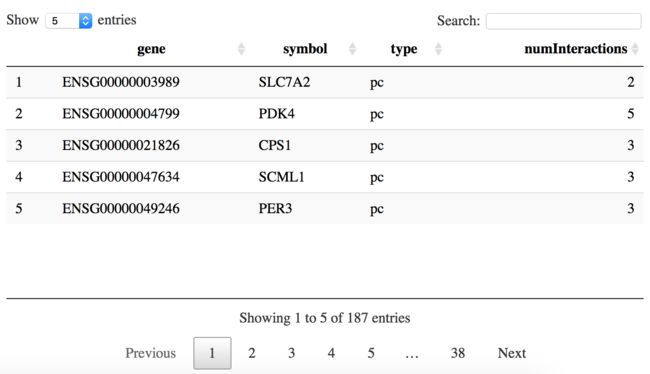
nodes <- gdcExportNetwork(ceNetwork = ceOutput2, net = 'nodes')
datatable(as.data.frame(nodes),
options = list(scrollX = TRUE, pageLength = 5))
Case study: TCGA-CHOL
下载RNA 和miRNA表达矩阵及临床信息:
####### Download RNAseq data #######
gdcRNADownload(project.id = 'TCGA-CHOL',
               data.type      = 'RNAseq',
               write.manifest = FALSE,
               method         = 'gdc-client',
               directory      = rnadir)
####### Download mature miRNA data #######
gdcRNADownload(project.id = 'TCGA-CHOL',
               data.type      = 'miRNAs',
               write.manifest = FALSE,
               method         = 'gdc-client',
               directory      = mirdir)
####### Download clinical data #######
clinicaldir <- paste(project, 'Clinical', sep='/')
gdcClinicalDownload(project.id = 'TCGA-CHOL',
                    write.manifest = FALSE,
                    method         = 'gdc-client',
                    directory      = clinicaldir)
自动下载网络可能不好,下载很慢,也可以手动下载:
用户可以从GDC cart下载 manifest file
- Step1: Download
GDC Data Transfer Toolon the GDC website - Step2: Add data to the GDC cart, then download manifest file and metadata of the cart
- Step3: Download data using
gdcRNADownload()orgdcClinicalDownload()functions by providing the manifest file
Data organization and DE analysis
临床信息来源可以是metadata file (.json) 从下载步骤自动下载的, 或者是
project.id和data.type通过gdcParseMetadata()函数从manifest file获取的诸如age, stage and gender等。只有一个样本最终会被保留,如果测序次数不只一次的情况下,过滤函数
gdcFilterDuplicate()做的这件事。样本既不是Primary Tumor (code: 01) 也不是Solid Tissue Normal (code: 11) 将会被
gdcFilterSampleType()函数过滤掉。
Parse metadata
####### Parse RNAseq metadata #######
metaMatrix.RNA <- gdcParseMetadata(project.id = 'TCGA-CHOL',
                                   data.type  = 'RNAseq',
                                   write.meta = FALSE)
####### Filter duplicated samples in RNAseq metadata #######
metaMatrix.RNA <- gdcFilterDuplicate(metaMatrix.RNA)
####### Filter non-Primary Tumor and non-Solid Tissue Normal samples in RNAseq metadata #######
metaMatrix.RNA <- gdcFilterSampleType(metaMatrix.RNA)
####### Parse miRNAs metadata #######
metaMatrix.MIR <- gdcParseMetadata(project.id = 'TCGA-CHOL',
                                   data.type  = 'miRNAs',
                                   write.meta = FALSE)
####### Filter duplicated samples in miRNAs metadata #######
metaMatrix.MIR <- gdcFilterDuplicate(metaMatrix.MIR)
####### Filter non-Primary Tumor and non-Solid Tissue Normal samples in miRNAs metadata #######
metaMatrix.MIR <- gdcFilterSampleType(metaMatrix.MIR)
Merge raw counts data
gdcRNAMerge()合并raw counts data of RNAseq到一个表达矩阵行是Ensembl id列是samples. miRNAs的5p 和3p分别来自isoform quantication文件和数据库miRBase v21. 如果数据样本来自不同的样本和不同的文件夹设置参数specify organized=FALSE此外设置specify organized=TRUE.
####### Merge RNAseq data #######
rnaCounts <- gdcRNAMerge(metadata  = metaMatrix.RNA,
                         path      = rnadir,
                         organized = FALSE, # if the data are in separate folders
                         data.type = 'RNAseq')
####### Merge miRNAs data #######
mirCounts <- gdcRNAMerge(metadata = metaMatrix.MIR,
                         path = mirdir, # the folder in which the data
                         organized = FALSE, # if the data are in separate folders
                         data.type = 'miRNAs')
Merge clinical data
设置参数key.info=TRUE, 仅common clinical信息可以被保留否则所有的clinical information从XML文件中被提取。
####### Merge clinical data #######
clinicalDa <- gdcClinicalMerge(path = clinicaldir, key.info = TRUE)
clinicalDa[1:6,5:10]
TMM normalization and voom transformation
edgeR(Robinson, McCarthy, and Smyth 2010) 中的函数TMM将raw counts进行normalized然后通过limma(Ritchie et al. 2015)函数进一步转换。低表达基因(logcpm < 1 in more than half of the samples)默认会被过滤掉。所有的基因可以通过设置gdcVoomNormalization()的参数filter=TRUE进行保留。
####### Normalization of RNAseq data #######
rnaExpr <- gdcVoomNormalization(counts = rnaCounts, filter = FALSE)
####### Normalization of miRNAs data #######
mirExpr <- gdcVoomNormalization(counts = mirCounts, filter = FALSE)
Dierential gene expression analysis
通常,人们对在不同组之间差异表达的基因感兴趣(eg. Primary Tumor vs. Solid Tissue Normal)。一种简易包装函数gdcDEAnalysis()来自limma, edgeR和 DESeq2用于获取差异基因(DEGs)或差异miRNAs。 注意,DESeq2对于单核处理器可能会很慢。 如果使用了DESeq2,则可以使用nCore参数指定多个内核。 鼓励用户查阅每种方法的vignette帮助文档,以获取更多详细信息。
DEGAll <- gdcDEAnalysis(counts = rnaCounts,
                        group = metaMatrix.RNA$sample_type,
                        comparison = 'PrimaryTumor-SolidTissueNormal',
                        method     = 'limma')
所有DEGs,DE长非编码基因,DE蛋白编码基因和DE miRNA都可以通过在gdcDEReport()中设置geneType参数来分别报告。 报告中输出了基于“ Ensembl 90”注释的Gene symbols和biotypes。
data(DEGAll)
### All DEGs
deALL <- gdcDEReport(deg = DEGAll, gene.type = 'all')
### DE long-noncoding
deLNC <- gdcDEReport(deg = DEGAll, gene.type = 'long_non_coding')
### DE protein coding genes
dePC <- gdcDEReport(deg = DEGAll, gene.type = 'protein_coding')
DEG visualization
火山图和条形图分别通过gdcVolcanoPlot()和gdcBarPlot()函数以不同的方式可视化DE分析结果。可以通过gdcHeatmap()函数分析和绘制DEGs表达矩阵的分层聚类。
Volcano plot,Barplot
a1 <- gdcVolcanoPlot(DEGAll)
a2 <- gdcBarPlot(deg = deALL, angle = 45, data.type = 'RNAseq')
library(patchwork)
a1+a2

Heatmap
热图是基于gplots包中的heatmap.2()函数生成的。
degName = rownames(deALL)
gdcHeatmap(deg.id = degName, metadata = metaMatrix.RNA, rna.expr = rnaExpr)

Competing endogenous RNAs network analysis
Three criteria are used to determine the competing endogenous interactions between lncRNA-mRNA pairs:
- The lncRNA and mRNA must share signicant number of miRNAs
- Expression of lncRNA and mRNA must be positively correlated
- Those common miRNAs should play similar roles in regulating the expression of lncRNA and mRNA
Hypergeometric test
超几何检验以测试lncRNA和mRNA是否显著共享许多miRNA。
新开发的算法spongeScan(Furi’o-Tar’i et al. 2016) 用于预测充当ceRNA的lncRNA中的MREs。 使用starBase v2.0(Li et al. 2014),miRcode(Jeggari, Marks, and Larsson 2012) and mirTarBase release 7.0(Chou et al. 2017)等数据库收集预测的和经过实验验证的miRNA-mRNA和/或 miRNA-lncRNA相互作用。 这些数据库中的基因ID已更新为人类基因组的最新Ensembl 90注释,而miRNA名称已更新为新版本的miRBase 21标识符。 用户还可以提供自己的miRNA-lncRNA和miRNA-mRNA相互作用数据集。

here m is the number of shared miRNAs, N is the total number of miRNAs in the database, n is the number of miRNAs targeting the lncRNA, K is the number of miRNAs targeting the protein coding gene.
Pearson correlation analysis
皮尔逊相关系数是两个变量之间线性关联强度的度量。 众所周知,miRNA是基因表达的负调控因子。 如果更多的常见miRNA被lncRNA占据,则它们中的更少将与靶mRNA结合,从而增加mRNA的表达水平。 因此,在ceRNA对中lncRNA和mRNA的表达应呈正相关。
Two methods are used to measure the regulatory role of miRNAs on the lncRNA and mRNA:
-
Regulation similarity
 image.png
 -
Sensitivity correlation
 image.png
看到公式头就晕,数学太差不想深究。暂时搁置。
ceRNAs network analysis
miRNA和lncRNA-mRNA共享的超几何检验的表达相关性分析及调控模式分析均已在gdcCEAnalysis()函数。
ceRNAs network analysis using internal databases
用户可以使用内部整合的miRNA-mRNA(starBase v2.0, miRcode, and mirTarBase v7.0)和miRNA-lncRNA(starBase v2.0, miRcode, spongeScan)交互的数据库来进行ceRNAs网络分析。
ceOutput <- gdcCEAnalysis(lnc = rownames(deLNC),
                          pc = rownames(dePC),
                          lnc.targets = 'starBase',
                          pc.targets  = 'starBase',
                          rna.expr    = rnaExpr,
                          mir.expr    = mirExpr)
ceRNAs network analysis using user-provided datasets
gdcCEAnalysis()还可以获取用户提供的miRNA-mRNA和miRNA-lncRNA相互作用数据集,例如TargetScan,miRanda和Diana Tools等预测的miRNA-靶标相互作用,用于ceRNAs网络分析。
### load miRNA-lncRNA interactions
data(lncTarget)
### load miRNA-mRNA interactions
data(pcTarget)
pcTarget[1:3]
ceOutput <- gdcCEAnalysis(lnc = rownames(deLNC),
                          pc = rownames(dePC),
                          lnc.targets = lncTarget,
                          pc.targets  = pcTarget,
                          rna.expr    = rnaExpr,
                          mir.expr    = mirExpr)
Network visulization in Cytoscape
lncRNA-miRNA-mRNA相互作用可以通过gdcExportNetwork()报告,并在Cytoscape中可视化。 应将edges作为网络导入,将节点作为特征表导入。
ceOutput2 <- ceOutput[ceOutput$hyperPValue<0.01 &
    ceOutput$corPValue<0.01 & ceOutput$regSim != 0,]

edges <- gdcExportNetwork(ceNetwork = ceOutput2, net = 'edges')
nodes <- gdcExportNetwork(ceNetwork = ceOutput2, net = 'nodes')

write.table(edges, file='edges.txt', sep='\t', quote=F)
write.table(nodes, file='nodes.txt', sep='\t', quote=F)
Correlation plot
gdcCorPlot(gene1 = 'ENSG00000251165',
           gene2 = 'ENSG00000091831',
           rna.expr = rnaExpr,
           metadata = metaMatrix.RNA)

Correlation plot on a local webpage
只需单击每个下拉框(in the GUI window)的基因,即可轻松操作基于shiny软件包的交互式绘图功能shinyCorPlot()。 通过运行使用shinyCorPlot()功能,将弹出一个本地网页,并自动显示lncRNA和mRNA之间的相关图。
shinyCorPlot(gene1 = rownames(deLNC),
             gene2 = rownames(dePC),
             rna.expr = rnaExpr,
             metadata = metaMatrix.RNA)

这个图很棒,可以随意挑选任意搭配。
Other downstream analyses
在GDCRNATools软件包中开发了下游分析,例如单变量生存分析和功能富集分析,以促进ceRNA网络中基因的鉴定,这些基因在预后中起重要作用或在重要途径中起作用。
Univariate survival analysis
提供了两种方法来执行单变量生存分析:Cox Proportional-Hazards (CoxPH) 模型和基于survival包的 Kaplan Meier (KM) 分析。 CoxPH模型将表达值视为连续变量,而KM分析通过用户定义的阈值(例如中位数或均值)将患者分为高表达和低表达组。gdcSurvivalAnalysis()将基因列表作为输入,并报告hazard ratio,95%的置信区间,并测试每种基因对总体存活率的影响。
CoxPH analysis
####### CoxPH analysis #######
survOutput <- gdcSurvivalAnalysis(gene = rownames(deALL),
                                  method   = 'coxph',
                                  rna.expr = rnaExpr,
                                  metadata = metaMatrix.RNA)
KM analysis
####### KM analysis #######
survOutput <- gdcSurvivalAnalysis(gene = rownames(deALL),
                                  method   = 'KM',
                                  rna.expr = rnaExpr,
                                  metadata = metaMatrix.RNA,
                                  sep      = 'median')
KM plot
gdcKMPlot(gene = 'ENSG00000136193',
          rna.expr = rnaExpr,
          metadata = metaMatrix.RNA,
          sep      = 'median')
KM plot on a local webpage by shinyKMPlot
The shinyKMPlot() function is also a simple shiny app which allow users view KM plots (based on the R package survminer.) of all genes of interests on a local webpackage conveniently.
shinyKMPlot(gene = rownames(deALL), rna.expr = rnaExpr,
            metadata = metaMatrix.RNA)

这里应该可以批量导出生存曲线了,也是挺不错的小工具。
Functional enrichment analysis
gdcEnrichAnalysis() can perform Gene ontology (GO), Kyoto Encyclopedia of Genes and Genomes (KEGG) and Disease Ontology (DO) functional enrichment analyses of a list of genes simultaneously. GO and KEGG analyses are based on the R/Bioconductor packages clusterProlier(Yu et al. 2012) and DOSE(Yu et al. 2015). Redundant GO terms can be removed by specifying simplify=TRUE in the gdcEnrichAnalysis() function which uses the simplify() function in the clusterProlier(Yu et al. 2012) package.
enrichOutput <- gdcEnrichAnalysis(gene = rownames(deALL), simplify = TRUE)
这一步做了5种富集分析,耗时有点长。
Barplot
data(enrichOutput)
gdcEnrichPlot(enrichOutput, type = 'bar', category = 'GO', num.terms = 10)

Bubble plot
gdcEnrichPlot(enrichOutput, type='bubble', category='GO', num.terms = 10)

View pathway maps on a local webpage
shinyPathview()allows users view and download pathways of interests by simply selecting the pathway terms on a local webpage.
library(pathview)
deg <- deALL$logFC
names(deg) <- rownames(deALL)
pathways <- as.character(enrichOutput$Terms[enrichOutput$Category=='KEGG'])
pathways
shinyPathview(deg, pathways = pathways, directory = 'pathview')
> pathways
 [1] "hsa05414~Dilated cardiomyopathy (DCM)"
 [2] "hsa05410~Hypertrophic cardiomyopathy (HCM)"
 [3] "hsa05412~Arrhythmogenic right ventricular cardiomyopathy (ARVC)"
 [4] "hsa04512~ECM-receptor interaction"
 [5] "hsa04510~Focal adhesion"
 [6] "hsa04360~Axon guidance"
 [7] "hsa04270~Vascular smooth muscle contraction"
 [8] "hsa05205~Proteoglycans in cancer"
 [9] "hsa04022~cGMP-PKG signaling pathway"
[10] "hsa00480~Glutathione metabolism"
sessionInfo
> sessionInfo()
R version 3.6.1 (2019-07-05)
Platform: x86_64-apple-darwin15.6.0 (64-bit)
Running under: macOS High Sierra 10.13.6

Matrix products: default
BLAS:   /System/Library/Frameworks/Accelerate.framework/Versions/A/Frameworks/vecLib.framework/Versions/A/libBLAS.dylib
LAPACK: /Library/Frameworks/R.framework/Versions/3.6/Resources/lib/libRlapack.dylib

locale:
[1] C

attached base packages:
[1] parallel  stats4    stats     graphics  grDevices utils     datasets
[8] methods   base

other attached packages:
[1] shiny_1.4.0          GDCRNATools_1.6.0    pathview_1.26.0
[4] org.Hs.eg.db_3.10.0  AnnotationDbi_1.48.0 IRanges_2.20.0
[7] S4Vectors_0.24.0     Biobase_2.46.0       BiocGenerics_0.32.0

loaded via a namespace (and not attached):
  [1] backports_1.1.5             Hmisc_4.2-0
  [3] fastmatch_1.1-0             BiocFileCache_1.10.0
  [5] plyr_1.8.4                  igraph_1.2.4.1
  [7] lazyeval_0.2.2              splines_3.6.1
  [9] BiocParallel_1.20.0         GenomeInfoDb_1.22.0
 [11] ggplot2_3.2.1               urltools_1.7.3
 [13] digest_0.6.23               htmltools_0.4.0
 [15] GOSemSim_2.12.0             rsconnect_0.8.15
 [17] viridis_0.5.1               GO.db_3.10.0
 [19] gdata_2.18.0                magrittr_1.5
 [21] checkmate_1.9.4             memoise_1.1.0
 [23] cluster_2.1.0               limma_3.42.0
 [25] Biostrings_2.54.0           readr_1.3.1
 [27] annotate_1.64.0             graphlayouts_0.5.0
 [29] matrixStats_0.55.0          askpass_1.1
 [31] enrichplot_1.6.0            prettyunits_1.0.2
 [33] colorspace_1.4-1            blob_1.2.0
 [35] rappdirs_0.3.1              ggrepel_0.8.1
 [37] xfun_0.10                   dplyr_0.8.3
 [39] crayon_1.3.4                RCurl_1.95-4.12
 [41] jsonlite_1.6                graph_1.64.0
 [43] genefilter_1.68.0           zeallot_0.1.0
 [45] zoo_1.8-6                   survival_2.44-1.1
 [47] glue_1.3.1                  survminer_0.4.6
 [49] GenomicDataCommons_1.10.0   polyclip_1.10-0
 [51] gtable_0.3.0                zlibbioc_1.32.0
 [53] XVector_0.26.0              DelayedArray_0.12.0
 [55] Rgraphviz_2.30.0            scales_1.1.0
 [57] DOSE_3.12.0                 DBI_1.0.0
 [59] edgeR_3.28.0                Rcpp_1.0.3
 [61] viridisLite_0.3.0           xtable_1.8-4
 [63] progress_1.2.2              htmlTable_1.13.2
 [65] gridGraphics_0.4-1          foreign_0.8-72
 [67] bit_1.1-14                  europepmc_0.3
 [69] km.ci_0.5-2                 Formula_1.2-3
 [71] DT_0.11                     htmlwidgets_1.5.1
 [73] httr_1.4.1                  fgsea_1.12.0
 [75] gplots_3.0.1.1              RColorBrewer_1.1-2
 [77] acepack_1.4.1               pkgconfig_2.0.3
 [79] XML_3.98-1.20               farver_2.0.1
 [81] nnet_7.3-12                 dbplyr_1.4.2
 [83] locfit_1.5-9.1              ggplotify_0.0.4
 [85] tidyselect_0.2.5            rlang_0.4.2
 [87] reshape2_1.4.3              later_1.0.0
 [89] munsell_0.5.0               tools_3.6.1
 [91] generics_0.0.2              RSQLite_2.1.2
 [93] broom_0.5.2                 ggridges_0.5.1
 [95] stringr_1.4.0               fastmap_1.0.1
 [97] yaml_2.2.0                  knitr_1.25
 [99] bit64_0.9-7                 tidygraph_1.1.2
[101] survMisc_0.5.5              caTools_1.17.1.2
[103] purrr_0.3.3                 KEGGREST_1.26.0
[105] ggraph_2.0.0                nlme_3.1-141
[107] mime_0.7                    KEGGgraph_1.46.0
[109] DO.db_2.9                   xml2_1.2.2
[111] biomaRt_2.42.0              compiler_3.6.1
[113] rstudioapi_0.10             png_0.1-7
[115] curl_4.2                    ggsignif_0.6.0
[117] tibble_2.1.3                tweenr_1.0.1
[119] geneplotter_1.64.0          stringi_1.4.3
[121] lattice_0.20-38             Matrix_1.2-17
[123] KMsurv_0.1-5                vctrs_0.2.0
[125] pillar_1.4.2                lifecycle_0.1.0
[127] BiocManager_1.30.9          triebeard_0.3.0
[129] data.table_1.12.6           cowplot_1.0.0
[131] bitops_1.0-6                httpuv_1.5.2
[133] GenomicRanges_1.38.0        qvalue_2.18.0
[135] R6_2.4.1                    latticeExtra_0.6-28
[137] promises_1.1.0              KernSmooth_2.23-16
[139] gridExtra_2.3               gtools_3.8.1
[141] MASS_7.3-51.4               assertthat_0.2.1
[143] SummarizedExperiment_1.16.0 rjson_0.2.20
[145] openssl_1.4.1               DESeq2_1.26.0
[147] GenomeInfoDbData_1.2.2      hms_0.5.2
[149] clusterProfiler_3.14.1      grid_3.6.1
[151] rpart_4.1-15                tidyr_1.0.0
[153] rvcheck_0.1.6               ggpubr_0.2.4
[155] ggforce_0.3.1               base64enc_0.1-3
这个教程还是非常有实用价值的。很多函数需要进一步理解,当然在学习这个教程之前最好还是先学习一下TCGA教程,不然有些不太容易理解。