4 TensorFlow进阶
4 TensorFlow进阶
4.1 合并与分割
合并是指将多个张量在某个维度上合并为一个张量。
张量A:shape为[2,2,3],张量B:shape为[3,2,3]
合并张量A与B,得到张量C:shape为[5,2,3]
张量的合并可以使用拼接(Concatenate)和堆(Stack)操作实现,拼接操作并不会产生新的维度,仅在现有的维度上合并,而堆叠会创建新维度。
拼接 拼接 在TensorFlow 中,可以通过tf.concat(tensors, axis) 函数拼接张量,其中
- 参数tensor保存了所有需要合并的张量List,
- 参数axis指定需要合并的维度索引
a = tf.random.normal([2,2,3])

b = tf.random.normal([3,2,3])

tf.concat([a,b], axis=0)
Out[4]:
<tf.Tensor: id=13, shape=(5, 2, 3), dtype=float32, numpy=
array([[[ 0.51841897,  0.25924757,  1.1976264 ],
        [-0.39768997, -0.4331023 ,  0.58553475]],

       [[ 0.8680533 , -0.765068  , -1.4970752 ],
        [ 1.4936122 , -0.25565544,  0.00814852]],

       [[ 0.5489708 , -0.44319677,  0.1148982 ],
        [ 2.195222  , -1.1085212 ,  1.3745565 ]],

       [[-0.17000443,  0.31869915,  0.72561115],
        [ 0.8638709 , -0.2608409 , -0.9443545 ]],

       [[ 1.1299909 ,  1.1774166 ,  0.27947757],
        [ 0.7602639 , -1.6035478 ,  1.7991685 ]]], dtype=float32)>
从语法上来说,拼接合并操作可以在任意的维度上进行,唯一的约束是非合并维度的长度必须一致
堆叠 使用 tf.stack(tensors, axis) 可以堆叠方式合并多个张量
- 参数tensors 列表表示将要合并的多个张量
- 参数axis 指定新维度插入的位置,axis 的用法与tf.expand_dims 的一致,当axis ≥ 0时,在axis之前插入;当axis < 0时,在axis 之后插入新维度
a = tf.constant([[1,2,3],[3,2,1]])

b = tf.constant([[4,5,6],[6,5,4]])

tf.stack([a,b], axis=0)
Out[7]:
<tf.Tensor: id=16, shape=(2, 2, 3), dtype=int32, numpy=
array([[[1, 2, 3],
        [3, 2, 1]],

       [[4, 5, 6],
        [6, 5, 4]]])>

tf.stack([a,b], axis=-1)
Out[8]:
<tf.Tensor: id=17, shape=(2, 3, 2), dtype=int32, numpy=
array([[[1, 4],
        [2, 5],
        [3, 6]],

       [[3, 6],
        [2, 5],
        [1, 4]]])>
分割 通过 tf.split(x, num_or_size_splits, axis) 可以完成张量的分割操作
- 参数x:待分割张量
- 参数num_or_size_splits:。当num_or_size_splits 为单个数值时,如10,表示等长切割为10 份;当num_or_size_splits 为List 时,List 的每个元素表示每份的长度,如[2,4,2,2]表示切割为4 份,每份的长度依次是2、4、2、2
- 参数axis指定分割的维度索引号
通过tf.unstack(x,axis) 函数切割长度固定为1,只需要指定切割维度的索引号
x = tf.random.normal([4,2,3])

result = tf.split(x, num_or_size_splits=[1,2,1], axis=0)

len(result)
Out[12]: 3

result[1]
Out[13]:
<tf.Tensor: id=29, shape=(2, 2, 3), dtype=float32, numpy=
array([[[ 0.12436184,  0.7961205 ,  0.33283442],
        [ 1.9214187 , -0.90878016,  1.2653215 ]],

       [[ 0.15603203,  0.4468012 ,  2.135242  ],
        [ 1.3672435 ,  0.7022418 ,  1.087458  ]]], dtype=float32)>

result = tf.unstack(x, axis=0)

len(result)
Out[15]: 4
4.2 数据统计
最值 最值位置 均值 范数–>张量数值分布
4.2.1 向量范数
向量范数Vecter Norm 常用来表示张量的权值大小,梯度大小等
- L1 范数 定义向量x的所有元素绝对值之和
∥ x ∥ 1 = ∑ i ∣ x i ∣ \|x\|_{1}=\sum_{i}\left|x_{i}\right| ∥x∥1=i∑∣xi∣ - L2 范数 定义向量x的所有元素的平方和,再开平方
∥ x ∥ 2 = ∑ i ∣ x i ∣ 2 \|x\|_{2}=\sqrt{\sum_{i}\left|x_{i}\right|^{2}} ∥x∥2=i∑∣xi∣2 - ∞ 范数 定义向量x的所有元素绝对值的最大值
∥ x ∥ ∞ = m a x i ( ∣ x i ∣ ) \|x\|_{\infty}=max _{i}\left(\left|x_{i}\right|\right) ∥x∥∞=maxi(∣xi∣)
对于矩阵和张量,同样可以利用向量范数的计算公式,等价于将矩阵和张量打平成向量后计算。
通过tf.norm(x, ord) 求解张量的L1、L2、∞等范数
参数ord 指定为1、2 时计算L1、L2 范数,指定为np.inf 时计算∞ 范数,
x = tf.ones([2,2])

tf.norm(x, ord=2)
Out[17]: <tf.Tensor: id=42, shape=(), dtype=float32, numpy=2.0>

tf.norm(x, ord=1)
Out[18]: <tf.Tensor: id=46, shape=(), dtype=float32, numpy=4.0>

tf.norm(x, ord=np.inf)
Out[20]: <tf.Tensor: id=50, shape=(), dtype=float32, numpy=1.0>
4.2.2 最值/均值/和
通过 tf.reduce_max、tf.reduce_min、tf.reduce_mean、tf.reduce_sum 函数可以求解张量在某个维度上的最大、最小、均值、和,也可以求全局最大、最小、均值、和
不指定axis 参数时,tf.reduce_* 函数会求解出全局元素的最大、最小、均值、和等数据
通过 tf.argmax(x, axis) 和tf.argmin(x, axis) 可以求解在axis 轴上,x 的最大值、最小值所在的索引号
4.3 张量比较
| 函数(a,b) | 逻辑 |
|---|---|
| tf.math.greater | a>b |
| tf.math.less | a |
| tf.math.greater_equal | a≥b |
| tf.math.less_equal | a≤b |
| tf.math.equal | a==b |
| tf.math.not_equal | a≠b |
| tf.math.is_nan | a==NaN |
4.4 填充与复制
4.4.1 填充
通过tf.pad(x, paddings) 函数实现
- 参数paddings 是包含了多个[Left Padding, Right Padding]的嵌套方案List,如[[0,0], [2,1], [1,2]]表示第一个维度不填充,第二个维度左边(起始处)填充两个单元,右边(结束处)填充一个单元,第三个维度左边填充一个单元,右边填充两个单元
a = tf.constant([1,2,3,4,5,6])

b = tf.constant([7,8,1,6])

b = tf.pad(b, [[0,2]])

b
Out[24]: <tf.Tensor: id=54, shape=(6,), dtype=int32, numpy=array([7, 8, 1, 6, 0, 0])>

tf.stack([a,b], axis=0)
Out[25]:
<tf.Tensor: id=55, shape=(2, 6), dtype=int32, numpy=
array([[1, 2, 3, 4, 5, 6],
       [7, 8, 1, 6, 0, 0]])>
4.4.2 复制
通过 tf.tile 函数可以在任意维度将数据重复复制多份,如shape 为[4,32,32,3]的数据,复制方案为multiples=[2,3,3,1],即通道数据不复制,高和宽方向分别复制2 份,图片数再复制1 份
4.5 数据限幅
通过tf.maximum(x, a)实现数据的下限幅,即
x ∈ [ a , + ∞ ) x \in[a,+\infty) x∈[a,+∞)
通过tf.minimum(x, a)实现数据的上限幅,即
x ∈ ( − ∞ , a ] x \in(-\infty, a] x∈(−∞,a]
通过tf.clip_by_value 函数实现上下限幅,即
x ∈ [ a , b ] x \in[a, b] x∈[a,b]
4.6 高级操作
4.6.1 tf.gather
tf.gather 可以实现根据索引号收集数据的目的。
x = tf.random.uniform([4,4,3], maxval=100, dtype=tf.int32)

tf.gather(x, [0,1], axis=0)
Out[48]:
<tf.Tensor: id=659558, shape=(2, 4, 3), dtype=int32, numpy=
array([[[76, 54, 46],
        [91,  9, 33],
        [52, 80, 68],
        [31, 65, 18]],

       [[ 8, 70, 46],
        [43, 75, 37],
        [30, 65, 64],
        [51, 92, 77]]])>

tf.gather(x, [0,2], axis=2)
Out[50]:
<tf.Tensor: id=659563, shape=(4, 4, 2), dtype=int32, numpy=
array([[[76, 46],
        [91, 33],
        [52, 68],
        [31, 18]],

       [[ 8, 46],
        [43, 37],
        [30, 64],
        [51, 77]],

       [[46, 64],
        [31, 16],
        [ 4, 90],
        [72, 75]],

       [[58,  9],
        [85, 59],
        [67,  1],
        [90, 20]]])>

tf.gather(tf.gather(x, [0,2], axis=2), [0,3], axis=0)
Out[51]:
<tf.Tensor: id=659569, shape=(2, 4, 2), dtype=int32, numpy=
array([[[76, 46],
        [91, 33],
        [52, 68],
        [31, 18]],

       [[58,  9],
        [85, 59],
        [67,  1],
        [90, 20]]])>
4.6.2 tf.gather_nd
通过tf.gather_nd 函数,可以通过指定每次采样点的多维坐标来实现采样多个点的目的。
x = tf.random.uniform([4,4,3], maxval=100, dtype=tf.int32)

tf.gather_nd(x, [[1,1],[3,3]])
Out[3]:
<tf.Tensor: id=5, shape=(2, 3), dtype=int32, numpy=
array([[ 6, 92, 85],
       [22,  6,  7]])>
4.6.3 tf.boolean_mask
通过给定掩码(Mask)和维度axis的方式进行采样
tf.boolean_mask(x,mask=[True,False,True,False],axis=0)
Out[4]:
<tf.Tensor: id=33, shape=(2, 4, 3), dtype=int32, numpy=
array([[[97, 77, 33],
        [78, 84, 68],
        [54, 90,  2],
        [99, 13, 72]],

       [[11, 43, 51],
        [23, 90, 23],
        [51,  1, 27],
        [21, 93, 53]]])>
注:掩码的长度必须与对应维度的长度一致
4.6.4 tf.where
通过 tf.where(cond, a, b)操作可以根据cond 条件的真假从参数A或B中读取数据,条件判定规则如下:
o_{i}=\left\{\begin{array}{ll}
{a_{i}} & {\text { cond }_{i}  \text {  is True }} \\
{b_{i}} & {\text { cond }_{i}  \text {  is False }}
\end{array}\right.
其中i为张量的元素索引,返回的张量大小与A和B一致,当对应位置的cond为True,从a中复制数据;当对应位置的cond为False,从b中复制数据
a = tf.ones([2,2])

b = tf.zeros([2,2])

cond = tf.constant([[True,False],[False,True]])

tf.where(cond,a,b)
Out[9]:
<tf.Tensor: id=41, shape=(2, 2), dtype=float32, numpy=
array([[1., 0.],
       [0., 1.]], dtype=float32)>
通过tf.where(cond)形式来获得每个True元素的索引坐标
tf.where(cond)
Out[10]:
<tf.Tensor: id=42, shape=(2, 2), dtype=int64, numpy=
array([[0, 0],
       [1, 1]], dtype=int64)>
4.6.5 tf.scatter_nd
通过 tf.scatter_nd(indices, updates, shape)函数可以高效地刷新张量的部分数据,但是这个函数只能在全0 的白板张量上面执行刷新操作
白板的形状通过shape 参数表示
需要刷新的数据索引号通过indices 表示
新数据为updates
根据indices 给出的索引位置将updates 中新的数据依次写入白板中,并返回更新后的结果张量。
indices = tf.constant([[4],[3],[1],[7]])

updates = tf.constant([4,3,1,7])

tf.scatter_nd(indices, updates, [8])
Out[13]: <tf.Tensor: id=46, shape=(8,), dtype=int32, numpy=array([0, 1, 0, 3, 4, 0, 0, 7])>
4.6.6 tf.meshgrid
通过 tf.meshgrid 函数可以方便地生成二维网格的采样点坐标,方便可视化等应用场合
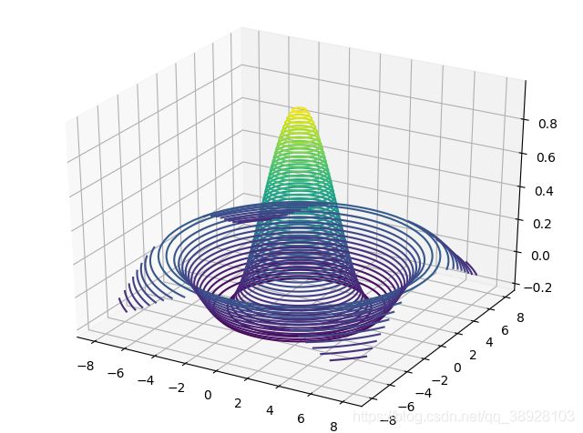
x = tf.linspace(-8.,8,100)

y = tf.linspace(-8.,8,100)

x,y = tf.meshgrid(x,y)

x.shape,y.shape
Out[17]: (TensorShape([100, 100]), TensorShape([100, 100]))

z = tf.sqrt(x**2+y**2)

z = tf.sin(z)/z

import matplotlib

from matplotlib import pyplot as plt

from mpl_toolkits.mplot3d import Axes3D

fig = plt.figure()

ax = Axes3D(fig)

ax.contour3D(x.numpy(), y.numpy(), z.numpy(), 50)
Out[26]: <matplotlib.contour.QuadContourSet at 0x1a3e651b648>
plt.show()
tf.linspace(start, end, num):这个函数主要的参数就这三个,start代表起始的值,end表示结束的值,num表示在这个区间里生成数字的个数,生成的数组是等间隔生成的。start和end这两个数字必须是浮点数,不能是整数
4.7 数据集加载
在 TensorFlow 中,keras.datasets 模块提供了常用经典数据集的自动下载、管理、加载与转换功能,并且提供了tf.data.Dataset 数据集对象,方便实现多线程(Multi-threading)、预处理(Preprocessing)、随机打散(Shuffle)和批训练(Training on Batch)等常用数据集的功能
通过 datasets.xxx.load_data()函数即可实现经典数据集的自动加载,其中xxx 代表具体的数据集名称,如“CIFAR10”、“MNIST”。TensorFlow 会默认将数据缓存在用户目录下的.keras/datasets 文件夹
from tensorflow.keras import  datasets

(x_train, y_train), (x_test, y_test) = datasets.mnist.load_data()

x_train.shape,y_train.shape,x_test.shape,y_test.shape
Out[31]: ((60000, 28, 28), (60000,), (10000, 28, 28), (10000,))
通过load_data()函数会返回2 个tuple,第一个tuple 保存了用于训练的数据x 和y 训练集对象;第2 个tuple 则保存了用于测试的数据x_test 和y_test 测试集对象,所有的数据都用Numpy 数组容器保存
数据加载进入内存后,需要转换成Dataset 对象,才能利用TensorFlow 提供的各种便捷功能。通过Dataset.from_tensor_slices 可以将训练部分的数据图片x 和标签y 都转换成Dataset 对象
train_db = tf.data.Dataset.from_tensor_slices((x_train,y_train))
4.7.1 随机打散
通过 Dataset.shuffle(buffer_size) 工具可以设置Dataset 对象随机打散数据之间的顺序,防止每次训练时数据按固定顺序产生
train_db = train_db.shuffle(10000)
buffer_size 参数指定缓冲池的大小,一般设置为一个较大的常数即可
4.7.2 批处理
为了利用显卡的并行计算能力,一般在网络的计算过程中会同时计算多个样本,这种训练方式叫做批训练,其中一个批中样本的数量叫做Batch Size
要设置Dataset 为批训练方式,Dataset 中产生Batch Size 数量的样本
train_db = train_db.batch(128)
4.7.3 预处理
Dataset 对象通过提供map(func)工具函数,可以非常方便地调用用户自定义的预处理逻辑,它实现在func 函数里
下方代码调用名为preprocess 的函数完成每个样本的预处理
train_db = train_db.map(preprocess)
preprocess函数实现
def preprocess(x,y):
    ...
    return x,y
4.7.4 循环训练
for epoch in range(20): # 训练Epoch 数
    for step, (x,y) in enumerate(train_db): # 迭代Step 数
        # training...
迭代数据集对象每次返回的x 和y 对象即为批量样本和标签。当对train_db 的所有样本完成一次迭代后,for 循环终止退出。这样完成一个Batch 的数据训练,叫做一个Step
通过多个step 来完成整个训练集的一次迭代,叫做一个Epoch
实际训练中迭代多个Epoch才能取得较好的训练效果