这部分教程依然来自Happy Belly Bioinformatics网站, 主要学习一下使用DADA2获得ASVs数据之后的进一步分析。譬如,微生物群落多样性,样品间的微生物群落差异分析以及系统进化等。
1. 工作环境设置和数据导入
> setwd("C:\\Users\\Administrator\\Documents\\R_work\\amplicon_example_workflow\\R_working_dir")
> getwd()
[1] "C:/Users/Administrator/Documents/R_work/amplicon_example_workflow/R_working_dir"
> list.files()
[1] "amplicon_example_analysis.R" "ASVs_counts.txt"
[3] "ASVs_taxonomy.txt"           "sample_info.txt"

#载入所需包
> library("phyloseq")
> library("vegan")
> library("DESeq2")
载入需要的程辑包:SummarizedExperiment
载入需要的程辑包:DelayedArray
载入需要的程辑包:matrixStats

载入程辑包:‘matrixStats’

The following objects are masked from ‘package:Biobase’:

    anyMissing, rowMedians

载入需要的程辑包:BiocParallel

载入程辑包:‘DelayedArray’

The following objects are masked from ‘package:matrixStats’:

    colMaxs, colMins, colRanges, rowMaxs, rowMins, rowRanges

The following objects are masked from ‘package:base’:

    aperm, apply

> library("ggplot2")
> library("dendextend")
> library("tidyr")
> library("viridis")
> library("reshape")

#导入数据
> count_tab <- read.table("ASVs_counts.txt", header=T, row.names=1, check.names=F)
> tax_tab <- as.matrix(read.table("ASVs_taxonomy.txt", header=T, row.names=1, check.names=F, na.strings="", sep="\t"))
> sample_info_tab <- read.table("sample_info.txt", header=T, row.names=1, check.names=F)
> sample_info_tab
      temp    type      char
B1       blank
B2       blank
B3       blank
B4       blank
BW1    2.0   water     water
BW2    2.0   water     water
R10   13.7    rock    glassy
R11    7.3    rock    glassy
R11BF  7.3 biofilm   biofilm
R12       rock   altered
R1A    8.6    rock   altered
R1B    8.6    rock   altered
R2     8.6    rock   altered
R3    12.7    rock   altered
R4    12.7    rock   altered
R5    12.7    rock   altered
R6    12.7    rock   altered
R7        rock carbonate
R8    13.5    rock    glassy
R9    13.7    rock    glassy
2. 数据清洗
# first we need to get a sum for each ASV across all 4 blanks and all 16 samples
blank_ASV_counts <- rowSums(count_tab[,1:4])
sample_ASV_counts <- rowSums(count_tab[,5:20])
blank_ASV_counts
sample_ASV_counts

# now we normalize them, here by dividing the samples' total by 4 ??? as there are 4x as many samples (16) as there are blanks (4)
norm_sample_ASV_counts <- sample_ASV_counts/4

# here we're getting which ASVs are deemed likely contaminants based on the threshold noted above:
blank_ASVs <- names(blank_ASV_counts[blank_ASV_counts * 10 > norm_sample_ASV_counts])
length(blank_ASVs) # this approach identified about 50 out of ~1550 that are likely to have orginated from contamination

# now we normalize them, here by dividing the samples' total by 4 ??? as there are 4x as many samples (16) as there are blanks (4)
norm_sample_ASV_counts <- sample_ASV_counts/4

# here we're getting which ASVs are deemed likely contaminants based on the threshold noted above:
blank_ASVs <- names(blank_ASV_counts[blank_ASV_counts * 10 > norm_sample_ASV_counts])

length(blank_ASVs) # this approach identified about 50 out of ~1550 that are likely to have orginated from contamination

# looking at the percentage of reads retained for each sample after removing these presumed contaminant ASVs shows that the blanks lost almost all of their sequences, while the samples, other than one of the bottom water samples, lost less than 1% of their sequences, as would be hoped
colSums(count_tab[!rownames(count_tab) %in% blank_ASVs, ]) / colSums(count_tab) * 100

# now that we've used our extraction blanks to identify ASVs that were likely due to contamination, we're going to trim down our count table by removing those sequences and the blank samples from further analysis
filt_count_tab <- count_tab[!rownames(count_tab) %in% blank_ASVs, -c(1:4)]

# and here make a filtered sample info table that doesn't contain the blanks
filt_sample_info_tab<-sample_info_tab[-c(1:4), ]

# and let's add some colors to the sample info table that are specific to sample types and characteristics that we will use when plotting things
# we'll color the water samples blue:
filt_sample_info_tab$color[filt_sample_info_tab$char == "water"] <- "blue"

# the biofilm sample a darkgreen:
filt_sample_info_tab$color[filt_sample_info_tab$char == "biofilm"] <- "darkgreen"

# the basalts with highly altered, thick outer rinds (>1 cm) brown ("chocolate4" is the best brown I can find...):
filt_sample_info_tab$color[filt_sample_info_tab$char == "altered"] <- "chocolate4"
# the basalts with smooth, glassy, thin exteriors black:
filt_sample_info_tab$color[filt_sample_info_tab$char == "glassy"] <- "black"
# and the calcified carbonate sample an ugly yellow:
filt_sample_info_tab$color[filt_sample_info_tab$char == "carbonate"] <- "darkkhaki"

# and now looking at our filtered sample info table we can see it has an addition column for color
filt_sample_info_tab
3. β多样性分析
主要计算样品之间的距离或者不同点,一般通过计算样品间的欧几里得距离来展示样品间的异同。但在不同样品的测序深度并不一致,这将影响欧几里得距离的计算,因此我们首先要将所有样品测序深度标准化。
一般的方法是,以最低测序深度样品为基准,将所有样品测序深度通过二次抽样调整到最低测序深度水平;或者是将每个样品测序的数量转化为比例值。作者这里推荐使用 DESeq2 包的来标准化样品数据。
# first we need to make a DESeq2 object
> deseq_counts <- DESeqDataSetFromMatrix(filt_count_tab, colData = filt_sample_info_tab, design = ~type)
> deseq_counts_vst <- varianceStabilizingTransformation(deseq_counts)
# pulling out our transformed table
> vst_trans_count_tab <- assay(deseq_counts_vst)
# and calculating our Euclidean distance matrix
> euc_dist <- dist(t(vst_trans_count_tab))
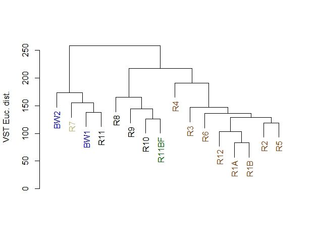
> euc_clust <- hclust(euc_dist, method="ward.D2")
# plot(euc_clust) # hclust objects like this can be plotted as is, but i like to change them to dendrograms for two reasons:
# 1) it's easier to color the dendrogram plot by groups
# 2) if you want you can rotate clusters with the rotate() function of the dendextend package
> euc_dend <- as.dendrogram(euc_clust, hang=0.1)
> dend_cols <- filt_sample_info_tab$color[order.dendrogram(euc_dend)]
> labels_colors(euc_dend) <- dend_cols
> plot(euc_dend, ylab="VST Euc. dist.")
根据样品间的欧几里德距离,对样品进行层次聚类。我作出来的跟作者的结果不完全一致,不知道问题出在哪儿。作者是使用Usearch分析得到的OTU数据,我是使用DADA2得到的ASVs数据,然后多样性的分析是参照的作者。可能是Usearch和DADA2分析结果不完全一致,也可能是我代码输入过程中出了一些未能察觉的差错导致的。
PCoA分析
> # making our phyloseq object with transformed table
> vst_count_phy <- otu_table(vst_trans_count_tab, taxa_are_rows=T)
> sample_info_tab_phy <- sample_data(filt_sample_info_tab)
> vst_physeq <- phyloseq(vst_count_phy, sample_info_tab_phy)
> # generating and visualizing the PCoA with phyloseq
> vst_pcoa <- ordinate(vst_physeq, method="MDS", distance="euclidean")
> eigen_vals <- vst_pcoa$values$Eigenvalues # allows us to scale the axes according to their magnitude of separating apart the samples
> plot_ordination(vst_physeq, vst_pcoa, color="char") +
+   labs(col="type") + geom_point(size=1) +
+   geom_text(aes(label=rownames(filt_sample_info_tab), hjust=0.3, vjust=-0.4)) +
+   coord_fixed(sqrt(eigen_vals[2]/eigen_vals[1])) + ggtitle("PCoA") +
+   scale_color_manual(values=unique(filt_sample_info_tab$color[order(filt_sample_info_tab$char)])) +
+   theme(legend.position="none")

结果依然跟作者不完全一致!
4. α多样性分析
样品稀薄曲线
> rarecurve(t(filt_count_tab), step=100, col=filt_sample_info_tab$color, lwd=2, ylab="ASVs")
abline(v=(min(rowSums(t(filt_count_tab)))))

群落丰富度和多样性计算
# first we need to create a phyloseq object using our un-transformed count table
> count_tab_phy <- otu_table(filt_count_tab, taxa_are_rows=T)
> tax_tab_phy <- tax_table(tax_tab)
> ASV_physeq <- phyloseq(count_tab_phy, tax_tab_phy, sample_info_tab_phy)
# first we need to create a phyloseq object using our un-transformed count table
> count_tab_phy <- otu_table(filt_count_tab1, taxa_are_rows=T)
> tax_tab_phy <- tax_table(tax_tab)
> ASV_physeq <- phyloseq(count_tab_phy, tax_tab_phy, sample_info_tab_phy)
# and now we can call the plot_richness() function on our phyloseq object
> plot_richness(ASV_physeq, color="char", measures=c("Chao1", "Shannon")) +
+   scale_color_manual(values=unique(filt_sample_info_tab$color[order(filt_sample_info_tab$char)])) +
+   theme(legend.title = element_blank())

phyloseq包绘图
> plot_richness(ASV_physeq, x="type", color="char", measures=c("Chao1", "Shannon")) +
+   scale_color_manual(values=unique(filt_sample_info_tab$color[order(filt_sample_info_tab$char)])) +
+   theme(legend.title = element_blank())

至此,16s扩增子的α和β多样性分析完成。我只是简单的过了一遍作者的流程和代码,其中的可视化部分还有待精雕细琢。下一步是微生物群落组成和丰度差异分析。