- 浏览器 DOM 深度解析:从节点类型到遍历操作的全攻略
码农的时光故事
javascript开发语言ecmascript
一、DOM核心概念与节点类型DOM(文档对象模型)是浏览器提供的核心API之一,用于将HTML文档转换为可操作的对象树结构。其核心设计遵循树形结构,每个节点都继承自Node接口,主要分为以下类型:1.基础节点类型Element:对应HTML标签,包含属性和子节点()Text:文本内容节点Comment:注释节点Document:文档根节点,通过document全局对象访问()2.特殊节点类型Doc
- 浏览器工作原理深度解析(阶段一):从 URL 到页面渲染的完整流程
码农的时光故事
javascript前端
一、浏览器工作流程概述作为前端开发者,我们每天都在与浏览器打交道,但多数人对其内部工作机制却知之甚少。实际上,浏览器的核心功能就是将用户输入的URL转换为可视化的网页。这一过程大致分为六个关键步骤:网络请求:通过HTTP/HTTPS协议获取页面资源构建DOM树:解析HTML代码生成文档对象模型样式计算:解析CSS规则并应用到对应元素布局渲染:计算元素位置和尺寸生成渲染树合成优化:将渲染层合并为位图
- 【MySQL必知必会】数据库操纵语言(DML)超全总结:增删改查一文搞定!
秀儿还能再秀
数据库MySQL学习笔记
一、DML简介数据库操纵语言(DataManipulationLanguage,DML)是SQL的核心组成部分,主要用于对数据库中的数据进行增(INSERT)、删(DELETE)、改(UPDATE)、查(SELECT)操作,掌握DML都是必备技能!二、核心操作详解1.插入数据:INSERT--插入单条数据(全字段)INSERTINTO表名VALUES(值1,值2,...);--指定字段插入INSE
- JAVA学习-练习试用Java实现“实现一个Spark应用,对大数据集中的文本数据进行情感分析和关键词筛选”
守护者170
java学习java学习
问题:实现一个Spark应用,对大数据集中的文本数据进行情感分析和关键词筛选。解答思路:要实现一个Spark应用,对大数据集中的文本数据进行情感分析和关键词筛选,需要按照以下步骤进行:1.环境准备确保的环境中已经安装了ApacheSpark。可以从[ApacheSpark官网](https://spark.apache.org/downloads.html)下载并安装。2.创建Spark应用以下是
- Bilibili 视频弹幕自动获取和自定义屏蔽词
dreadp
音视频htmlpythonjson前端自动化
脚本地址:项目地址:GazerdmGrab.py提要适用于:任意B站视频弹幕XML文件下载.如不能,请提交issues联系我.支持指定屏蔽词.1秒即可完成自动解析任意B站视频的视频弹幕XML文件请求链接,并下载.使用方法克隆或下载项目代码。安装依赖:pipinstallrequestslxml,或者克隆项目代码后pipinstall-rrequirements.txt脚本顶部:指定常量FOLDER
- pear-admin-boot开发框架使用记录(三)
后青春期的诗go
经验分享javaspringbootspringlog4jmybatis
一、实现部门选择操作用于从组织架构里选择出部门的操作,如开发日志管理模块,创建人新增日志时可以通过选择框选择相应共享的部门。数据库表调整在数据表添加2个字段:sharedeptid共享部门idvarcharsharedeptname共享部门名称varchar前端html页面调整页面添加如下代码:共享部门前端JS调整添加如下代码:letdtree=layui.dtree;dtree.renderSe
- python中的构造函数
weixin_30770495
python
python中构造函数可以这样写classclassname():def——init——(self):#构造函数函数体转载于:https://www.cnblogs.com/begoogatprogram/p/4649076.html
- HBuilderX的下载、安装
听海边涛声
HBuilderX
HBuilderX简称HX,是一款轻量级的、免费的IDE。它具有强大的语法提示和vue支持。访问HBuilderX的官网:https://www.dcloud.io/hbuilderx.html选择要下载的版本,我下载的是v4.08版本:将压缩包下拉以后解压到某个目录下就可以了,不需要安装过程,例如,我解压到D:\HBuilderX目录下面:双击HBuilderX.exe,就可以运行了:注意:HB
- 【BERT和GPT的区别】
调皮的芋头
人工智能深度学习机器学习bertgpt
BERT采用完形填空(MaskedLanguageModeling,MLM)与GPT采用自回归生成(AutoregressiveGeneration)的差异,本质源于两者对语言建模的不同哲学导向与技术目标的根本分歧。这种选择不仅塑造了模型的架构特性,更决定了其应用边界与能力上限。以下从语言建模本质、任务适配性、技术约束及后续影响四个维度深入剖析:一、语言建模的本质差异1.BERT的“全知视角”与全
- 微信小程序云开发实现登录功能
Bilkan-studio
微信小程序小程序前端
使用云开发数据库实现登录功能,多的不说了直接看代码登录功能代码段WXML代码账号密码登录WXSS代码page{width:100%;height:100%;direction:ltr;}.waikuang{width:100%;height:100%;display:flex;align-items:center;justify-content:center;flex-direction:colu
- python 读取配置文件
Pure Ven
python编程语言python
Python读取配置文件并打印文件信息配置文件field_len.conf内容为:[ddl_max_len]NUMBER_MAX_LEN=10VARCHAR2_MAX_LEN=1024[dml_max_len]NUMBER_MAX_LEN=10VARCHAR2_MAX_LEN=1024BLOB_MAX_LEN=500MFLOAT_MAX_LEN=P20S8DATE=12TIMESTAMP(6)=1
- hive 使用oracle数据库
sardtass
hadoophive开源项目
hive使用oracle作为数据源,导入数据使用sqoop或kettle或自己写代码(淘宝的开源项目中有一个xdata就是淘宝自己写的)。感觉sqoop比kettle快多了,淘宝的xdata没用过。hive默认使用derby作为存储表信息的数据库,默认在哪启动就在哪建一个metadata_db文件放数据,可以在conf下的hive-site.xml中配置为一个固定的位置,这样不论在哪启动都可以了。
- C1-Week2 Program Assignment: Logistic Regression with a Neural Network mindset
houzhizhen
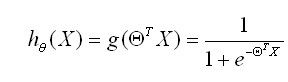
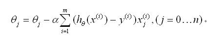
LogisticRegressionwithaNeuralNetworkmindsetWelcometoyourfirst(required)programmingassignment!Youwillbuildalogisticregressionclassifiertorecognizecats.ThisassignmentwillstepyouthroughhowtodothiswithaNe
- python读取配置参数的多种方式
WYRM_GOLD
python
使用多个配置文件:根据不同的环境(如开发、测试、生产)使用不同的配置文件。使用环境变量:利用操作系统的环境变量来获取参数。使用命令行参数:根据传入的命令行参数选择配置。使用JSON或YAML文件:配置文件可以使用JSON或YAML格式,支持多种环境的变量。方法1、使用多个配置文件假设有两个配置文件:config_dev.ini和config_prod.ini。config_dev.ini:[DEF
- Pybind11教程:从零开始打造 Python 的 C++ 小帮手
Yc9801
c++开发语言
参考官网文档:https://pybind11.readthedocs.io/en/stable/index.html一、Pybind11是什么?想象你在Python里写了个计算器,但跑得太慢,想用C++提速,又不想完全抛弃Python。Pybind11就像一座桥,把C++的高性能代码“嫁接”到Python里。你可以用Python调用C++函数,就像请了个跑得飞快的帮手来干活。主要功能:绑定函数:
- HTML 教程:从零开始掌握常用语法
LoveYa!
前端html前端笔记学习
免费无广纯净版微信小程序测mbti很有趣,不需要任何授权,也不需要登录,直接就是测,几分钟了解自己的人格mbti,快来试试吧。可以微信直接搜索小程序名“一秒MBTI”HTML教程:从零开始掌握常用语法欢迎来到HTML的世界!HTML(HyperTextMarkupLanguage,超文本标记语言)是网页开发的基石,它负责定义网页的结构和内容。无论你是想成为一名前端开发者,还是仅仅想了解网页背后的魔
- Spring Boot项目开发常见问题及解决方案(上)
小芬熊
面试学习路线阿里巴巴springboot后端java
启动相关问题问题1:项目启动时报错“找不到主类”在使用SpringBoot打包成可执行JAR文件后启动,有时会遇到这个头疼的问题。通常是因为打包配置有误或者项目结构不符合要求。解决方案:首先,检查pom.xml(Maven项目)或build.gradle(Gradle项目)中的打包插件配置。确保spring-boot-maven-plugin(Maven示例)配置正确,比如:org.springf
- Kotlin第十六讲---实战通过委托完成SharedPreferences封装
奇舞移动
jscssjava编程语言javascript
内容简介前面讲解了Kotlin具有类委托和属性委托。接下来我给大家分享1个实战技巧,使用属性委托来完成SharedPreferences的封装。前景介绍说起SharedPreferences在Android中是一种常用的本地化存储数据的方案。以前Java封装都是将SharedPreferences封装成单利,原因就是SharedPreferences对象创建过程会解析xml文件,这个过程比较耗性能
- vue3+Ts+elementPlus二次封装Table分页表格,表格内展示图片、switch开关、支持
龙井>_<
vue.js前端javascriptelementPlus
目录一.项目文件结构二.实现代码1.子组件(表格组件)2.父组件(使用表格)一.项目文件结构1.表格组件(子组件)位置2.使用表格组件的页面文件(父组件)位置3.演示图片位置elementPlus表格Table表格|ElementPlus4.笑果演示表格笑果点击图片放大显示笑果二.实现代码1.子组件(表格组件)1.src/views/Table.vuehtml部分{{scope.$index+1}
- 使用opengl绘制立方体_一步步学OpenGL(25) -《Skybox天空盒子》
weixin_39962153
使用opengl绘制立方体
教程25Skybox天空盒子原文:http://ogldev.atspace.co.uk/www/tutorial25/tutorial25.htmlCSDN完整版专栏:https://blog.csdn.net/cordova/article/category/9266966背景天空盒子是一种让场景看上去更广阔无垠的一种视觉技术,用无缝对接的封闭纹理将摄像机的视口360度无死角的包裹起来。封闭纹
- 下一代模型技术演进与场景应用突破
智能计算研究中心
其他
内容概要当前模型技术正经历多维度的范式跃迁,可解释性模型与自动化机器学习(AutoML)成为突破传统黑箱困境的核心路径。在底层架构层面,边缘计算与量子计算的融合重构了算力分配模式,联邦学习技术则为跨域数据协作提供了安全可信的解决方案。主流框架如TensorFlow和PyTorch持续迭代优化能力,通过动态参数压缩与自适应超参数调优策略,显著提升模型部署效率。应用层创新呈现垂直化特征,医疗诊断模型通
- Qwen2-Audio:通义千问音频大模型技术解读
kakaZhui
音视频AIGC人工智能pythonchatgpt
引言:从llm到mlm(audio)大型语言模型(LLM)的发展日新月异,它们在文本理解、生成、推理等方面展现出惊人的能力。然而,交互模态不仅仅依赖于文字,语音、语调、环境音等听觉信息同样承载着丰富的内容。阿里巴巴通义千问团队,推出了Qwen-Audio系列模型,这里我们一起看下最新版本Qwen2-Audio。Qwen2-Audio不仅能够理解各种音频信号,还能根据语音指令做出文本回应,甚至可以进
- 01.AJAX 概念和 axios 使用
Lv547
#AJAXajax前端javascript
01.AJAX概念和axios使用1.什么是AJAX?使用浏览器的XMLHttpRequest对象与服务器通信浏览器网页中,使用AJAX技术(XHR对象)发起获取省份列表数据的请求,服务器代码响应准备好的省份列表数据给前端,前端拿到数据数组以后,展示到网页2.什么是服务器?可以暂时理解为提供数据的一台电脑3.为何学AJAX?以前我们的数据都是写在代码里固定的,无法随时变化现在我们的数据可以从服务器
- 一种基于swagger 2.0 yaml文件的接口异常用例生成算法,单因子变量法
xiyubaby.17
java测试用例
详细解决方案一、设计思路基于Swagger2.0的YAML定义,为每个参数生成两类测试用例:正常用例:所有参数均符合约束。异常用例:仅一个参数违反约束,其他参数正常,且每个参数需覆盖所有可能的异常场景。二、实现步骤解析Swagger文件使用SnakeYAML解析YAML,提取参数定义(类型、约束、是否必填等)。生成正常值根据参数类型和约束生成合法值。生成异常值针对每个参数的所有约束,生成违反每个约
- 深入理解Ajax原理
lfsf802
前端技术ajaxxmlhttprequestjavascript服务器asynchronous
1.概念ajax的全称是AsynchronousJavaScriptandXML,其中,Asynchronous是异步的意思,它有别于传统web开发中采用的同步的方式。2.理解同步异步异步传输是面向字符的传输,它的单位是字符;而同步传输是面向比特的传输,它的单位是桢,它传输的时候要求接受方和发送方的时钟是保持一致的。举个例子来说同步和异步,同步就好像我们买楼一次性支付,而异步就是买楼分期付款。所以
- 【 <二> 丹方改良:Spring 时代的 JavaWeb】之 Spring MVC 的核心组件:DispatcherServlet 的工作原理
Foyo Designer
springmvcjavaservletHandlerMappingViewResolver
点击此处查看合集https://blog.csdn.net/foyodesigner/category_12907601.html?fromshare=blogcolumn&sharetype=blogcolumn&sharerId=12907601&sharerefer=PC&sharesource=FoyoDesigner&sharefrom=from_link一、DispatcherServ
- 【脑洞小剧场】零帧起手创业小公司之 第一次技术分享会
Foyo Designer
技术职场小剧职场和发展程序人生学习方法改行学it程序员创富
点击查看小剧场合集https://blog.csdn.net/foyodesigner/category_12896948.html阳光明媚的早晨,段萌儿怀揣着对新工作的无限憧憬,踏入了这家充满未知的小公司。然而,她万万没想到,第一天上班就迎来了一场“惊悚”之旅。阳光透过会议室的窗户,洒在摆满椅子的地板上,技术分享会的氛围既紧张又期待。今天,将是公司第一次正式的技术交流盛会,各路技术大牛摩拳擦掌,
- springboot使用163发送自定义html格式的邮件
星月前端
springboothtmljava
springboot使用163发送html格式的邮件效果:下面直接开始教学注册邮箱,生成授权码获取163邮箱的授权码,可以按照以下步骤操作:登录163邮箱打开浏览器,访问163邮箱登录页面。使用你的邮箱账号和密码登录。进入邮箱设置登录后,点击页面右上角的“设置”图标(通常是一个齿轮图标)。在菜单中选择“POP3/SMTP/IMAP”选项。开启SMTP服务在“POP3/SMTP/IMAP”设置页面中
- bitset and valarray
heraldww
c++数学ARMandroid漂亮的UI界面完整的界面设计职场和发展程序人生
记录一个比较少用的容器C++std::bitsethttps://www.cnblogs.com/wangshaowei/p/10297877.htmlvalarrayvalarray面向数值计算的数组,在C++11中才支持支持很多数值数组操作,如求数组总和、最大数、最小数等。需要头文件valarray支持
- 前端性能优化之SSR优化
xiangzhihong8
前端前端
我们常说的SSR是指Server-SideRendering,即服务端渲染,属于首屏直出渲染的一种方案。SSR也是前端性能优化中最常用的技术方案了,能有效地缩短页面的可见时间,给用户带来很好的体验。SSR渲染方案一般来说,我们页面加载会分为好几个步骤:请求域名,服务器返回HTML资源。浏览器加载HTML片段,识别到有CSS/JavaScript资源时,获取资源并加载。现在大多数前端页面都是单页面应
- 戴尔笔记本win8系统改装win7系统
sophia天雪
win7戴尔改装系统win8
戴尔win8 系统改装win7 系统详述
第一步:使用U盘制作虚拟光驱:
1)下载安装UltraISO:注册码可以在网上搜索。
2)启动UltraISO,点击“文件”—》“打开”按钮,打开已经准备好的ISO镜像文
- BeanUtils.copyProperties使用笔记
bylijinnan
java
BeanUtils.copyProperties VS PropertyUtils.copyProperties
两者最大的区别是:
BeanUtils.copyProperties会进行类型转换,而PropertyUtils.copyProperties不会。
既然进行了类型转换,那BeanUtils.copyProperties的速度比不上PropertyUtils.copyProp
- MyEclipse中文乱码问题
0624chenhong
MyEclipse
一、设置新建常见文件的默认编码格式,也就是文件保存的格式。
在不对MyEclipse进行设置的时候,默认保存文件的编码,一般跟简体中文操作系统(如windows2000,windowsXP)的编码一致,即GBK。
在简体中文系统下,ANSI 编码代表 GBK编码;在日文操作系统下,ANSI 编码代表 JIS 编码。
Window-->Preferences-->General -
- 发送邮件
不懂事的小屁孩
send email
import org.apache.commons.mail.EmailAttachment;
import org.apache.commons.mail.EmailException;
import org.apache.commons.mail.HtmlEmail;
import org.apache.commons.mail.MultiPartEmail;
- 动画合集
换个号韩国红果果
htmlcss
动画 指一种样式变为另一种样式 keyframes应当始终定义0 100 过程
1 transition 制作鼠标滑过图片时的放大效果
css
.wrap{
width: 340px;height: 340px;
position: absolute;
top: 30%;
left: 20%;
overflow: hidden;
bor
- 网络最常见的攻击方式竟然是SQL注入
蓝儿唯美
sql注入
NTT研究表明,尽管SQL注入(SQLi)型攻击记录详尽且为人熟知,但目前网络应用程序仍然是SQLi攻击的重灾区。
信息安全和风险管理公司NTTCom Security发布的《2015全球智能威胁风险报告》表明,目前黑客攻击网络应用程序方式中最流行的,要数SQLi攻击。报告对去年发生的60亿攻击 行为进行分析,指出SQLi攻击是最常见的网络应用程序攻击方式。全球网络应用程序攻击中,SQLi攻击占
- java笔记2
a-john
java
类的封装:
1,java中,对象就是一个封装体。封装是把对象的属性和服务结合成一个独立的的单位。并尽可能隐藏对象的内部细节(尤其是私有数据)
2,目的:使对象以外的部分不能随意存取对象的内部数据(如属性),从而使软件错误能够局部化,减少差错和排错的难度。
3,简单来说,“隐藏属性、方法或实现细节的过程”称为——封装。
4,封装的特性:
4.1设置
- [Andengine]Error:can't creat bitmap form path “gfx/xxx.xxx”
aijuans
学习Android遇到的错误
最开始遇到这个错误是很早以前了,以前也没注意,只当是一个不理解的bug,因为所有的texture,textureregion都没有问题,但是就是提示错误。
昨天和美工要图片,本来是要背景透明的png格式,可是她却给了我一个jpg的。说明了之后她说没法改,因为没有png这个保存选项。
我就看了一下,和她要了psd的文件,还好我有一点
- 自己写的一个繁体到简体的转换程序
asialee
java转换繁体filter简体
今天调研一个任务,基于java的filter实现繁体到简体的转换,于是写了一个demo,给各位博友奉上,欢迎批评指正。
实现的思路是重载request的调取参数的几个方法,然后做下转换。
- android意图和意图监听器技术
百合不是茶
android显示意图隐式意图意图监听器
Intent是在activity之间传递数据;Intent的传递分为显示传递和隐式传递
显式意图:调用Intent.setComponent() 或 Intent.setClassName() 或 Intent.setClass()方法明确指定了组件名的Intent为显式意图,显式意图明确指定了Intent应该传递给哪个组件。
隐式意图;不指明调用的名称,根据设
- spring3中新增的@value注解
bijian1013
javaspring@Value
在spring 3.0中,可以通过使用@value,对一些如xxx.properties文件中的文件,进行键值对的注入,例子如下:
1.首先在applicationContext.xml中加入:
<beans xmlns="http://www.springframework.
- Jboss启用CXF日志
sunjing
logjbossCXF
1. 在standalone.xml配置文件中添加system-properties:
<system-properties> <property name="org.apache.cxf.logging.enabled" value=&
- 【Hadoop三】Centos7_x86_64部署Hadoop集群之编译Hadoop源代码
bit1129
centos
编译必需的软件
Firebugs3.0.0
Maven3.2.3
Ant
JDK1.7.0_67
protobuf-2.5.0
Hadoop 2.5.2源码包
Firebugs3.0.0
http://sourceforge.jp/projects/sfnet_findbug
- struts2验证框架的使用和扩展
白糖_
框架xmlbeanstruts正则表达式
struts2能够对前台提交的表单数据进行输入有效性校验,通常有两种方式:
1、在Action类中通过validatexx方法验证,这种方式很简单,在此不再赘述;
2、通过编写xx-validation.xml文件执行表单验证,当用户提交表单请求后,struts会优先执行xml文件,如果校验不通过是不会让请求访问指定action的。
本文介绍一下struts2通过xml文件进行校验的方法并说
- 记录-感悟
braveCS
感悟
再翻翻以前写的感悟,有时会发现自己很幼稚,也会让自己找回初心。
2015-1-11 1. 能在工作之余学习感兴趣的东西已经很幸福了;
2. 要改变自己,不能这样一直在原来区域,要突破安全区舒适区,才能提高自己,往好的方面发展;
3. 多反省多思考;要会用工具,而不是变成工具的奴隶;
4. 一天内集中一个定长时间段看最新资讯和偏流式博
- 编程之美-数组中最长递增子序列
bylijinnan
编程之美
import java.util.Arrays;
import java.util.Random;
public class LongestAccendingSubSequence {
/**
* 编程之美 数组中最长递增子序列
* 书上的解法容易理解
* 另一方法书上没有提到的是,可以将数组排序(由小到大)得到新的数组,
* 然后求排序后的数组与原数
- 读书笔记5
chengxuyuancsdn
重复提交struts2的token验证
1、重复提交
2、struts2的token验证
3、用response返回xml时的注意
1、重复提交
(1)应用场景
(1-1)点击提交按钮两次。
(1-2)使用浏览器后退按钮重复之前的操作,导致重复提交表单。
(1-3)刷新页面
(1-4)使用浏览器历史记录重复提交表单。
(1-5)浏览器重复的 HTTP 请求。
(2)解决方法
(2-1)禁掉提交按钮
(2-2)
- [时空与探索]全球联合进行第二次费城实验的可能性
comsci
二次世界大战前后,由爱因斯坦参加的一次在海军舰艇上进行的物理学实验 -费城实验
至今给我们大家留下很多迷团.....
关于费城实验的详细过程,大家可以在网络上搜索一下,我这里就不详细描述了
在这里,我的意思是,现在
- easy connect 之 ORA-12154: TNS: 无法解析指定的连接标识符
daizj
oracleORA-12154
用easy connect连接出现“tns无法解析指定的连接标示符”的错误,如下:
C:\Users\Administrator>sqlplus username/
[email protected]:1521/orcl
SQL*Plus: Release 10.2.0.1.0 – Production on 星期一 5月 21 18:16:20 2012
Copyright (c) 198
- 简单排序:归并排序
dieslrae
归并排序
public void mergeSort(int[] array){
int temp = array.length/2;
if(temp == 0){
return;
}
int[] a = new int[temp];
int
- C语言中字符串的\0和空格
dcj3sjt126com
c
\0 为字符串结束符,比如说:
abcd (空格)cdefg;
存入数组时,空格作为一个字符占有一个字节的空间,我们
- 解决Composer国内速度慢的办法
dcj3sjt126com
Composer
用法:
有两种方式启用本镜像服务:
1 将以下配置信息添加到 Composer 的配置文件 config.json 中(系统全局配置)。见“例1”
2 将以下配置信息添加到你的项目的 composer.json 文件中(针对单个项目配置)。见“例2”
为了避免安装包的时候都要执行两次查询,切记要添加禁用 packagist 的设置,如下 1 2 3 4 5
- 高效可伸缩的结果缓存
shuizhaosi888
高效可伸缩的结果缓存
/**
* 要执行的算法,返回结果v
*/
public interface Computable<A, V> {
public V comput(final A arg);
}
/**
* 用于缓存数据
*/
public class Memoizer<A, V> implements Computable<A,
- 三点定位的算法
haoningabc
c算法
三点定位,
已知a,b,c三个顶点的x,y坐标
和三个点都z坐标的距离,la,lb,lc
求z点的坐标
原理就是围绕a,b,c 三个点画圆,三个圆焦点的部分就是所求
但是,由于三个点的距离可能不准,不一定会有结果,
所以是三个圆环的焦点,环的宽度开始为0,没有取到则加1
运行
gcc -lm test.c
test.c代码如下
#include "stdi
- epoll使用详解
jimmee
clinux服务端编程epoll
epoll - I/O event notification facility在linux的网络编程中,很长的时间都在使用select来做事件触发。在linux新的内核中,有了一种替换它的机制,就是epoll。相比于select,epoll最大的好处在于它不会随着监听fd数目的增长而降低效率。因为在内核中的select实现中,它是采用轮询来处理的,轮询的fd数目越多,自然耗时越多。并且,在linu
- Hibernate对Enum的映射的基本使用方法
linzx0212
enumHibernate
枚举
/**
* 性别枚举
*/
public enum Gender {
MALE(0), FEMALE(1), OTHER(2);
private Gender(int i) {
this.i = i;
}
private int i;
public int getI
- 第10章 高级事件(下)
onestopweb
事件
index.html
<!DOCTYPE html PUBLIC "-//W3C//DTD XHTML 1.0 Transitional//EN" "http://www.w3.org/TR/xhtml1/DTD/xhtml1-transitional.dtd">
<html xmlns="http://www.w3.org/
- 孙子兵法
roadrunners
孙子兵法
始计第一
孙子曰:
兵者,国之大事,死生之地,存亡之道,不可不察也。
故经之以五事,校之以计,而索其情:一曰道,二曰天,三曰地,四曰将,五
曰法。道者,令民于上同意,可与之死,可与之生,而不危也;天者,阴阳、寒暑
、时制也;地者,远近、险易、广狭、死生也;将者,智、信、仁、勇、严也;法
者,曲制、官道、主用也。凡此五者,将莫不闻,知之者胜,不知之者不胜。故校
之以计,而索其情,曰
- MySQL双向复制
tomcat_oracle
mysql
本文包括:
主机配置
从机配置
建立主-从复制
建立双向复制
背景
按照以下简单的步骤:
参考一下:
在机器A配置主机(192.168.1.30)
在机器B配置从机(192.168.1.29)
我们可以使用下面的步骤来实现这一点
步骤1:机器A设置主机
在主机中打开配置文件 ,
- zoj 3822 Domination(dp)
阿尔萨斯
Mina
题目链接:zoj 3822 Domination
题目大意:给定一个N∗M的棋盘,每次任选一个位置放置一枚棋子,直到每行每列上都至少有一枚棋子,问放置棋子个数的期望。
解题思路:大白书上概率那一张有一道类似的题目,但是因为时间比较久了,还是稍微想了一下。dp[i][j][k]表示i行j列上均有至少一枚棋子,并且消耗k步的概率(k≤i∗j),因为放置在i+1~n上等价与放在i+1行上,同理