背景:
1.1 最早是由 Vladimir N. Vapnik 和 Alexey Ya. Chervonenkis 在1963年提出
1.2 目前的版本(soft margin)是由Corinna Cortes 和 Vapnik在1993年提出,并在1995年发表
1.3 深度学习(2012)出现之前,SVM被认为机器学习中近十几年来最成功,表现最好的算法
机器学习的一般框架:
训练集 => 提取特征向量 => 结合一定的算法(分类器:比如决策树,KNN)=>得到结果
介绍:
3.1 例子:
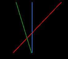
两类?哪条线最好?
SVM寻找区分两类的超平面(hyper plane), 使边际(margin)最大

总共可以有多少个可能的超平面?无数条
如何选取使边际(margin)最大的超平面 (Max Margin Hyperplane)?
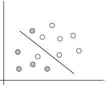
超平面到一侧最近点的距离等于到另一侧最近点的距离,两侧的两个超平面平行
线性可区分(linear separable) 和 线性不可区分 (linear inseparable)


定义与公式建立
超平面可以定义为n 是特征值的个数
X: 训练实例
b: bias

假设2维特征向量:X = (x1, X2)
把 b 想象为额外的 wight
超平面方程变为:调整weight,使超平面定义边际的两边:
综合以上两式,得到: yi(w0 + w1x1 + w2x2) >=1,任意i. (1)
所有坐落在边际的两边的超平面上的点被称作“支持向量(support vectors)”
分界的超平面到H1或H2上任意一点的距离为:
是向量的范数(norm))
求解
SVM如何找出最大边际的超平面呢(MMH)?
利用一些数学推倒,以上公式(1)可变为有限制的凸优化问题(convex quadratic optimization)
利用Karush-Kuhn-Tucker(KKT)条件和拉格朗日公式,可以推出MMH可以被表示为以下“决定边界”(decision boundary)
其中,yi是支持向量点Xi(support vector)的类别标记(class lable)
是要测试的实例
和 b0 都是单一数值型参数,由以上提到的最优算法得出
l 是支持向量点的个数
对于任何测试(要归类的)实例,带入以上公式,得出的符号是正还是负决定
例子:


说明:(2,3)减去(1,1)可以把weight表示为 (a,2a)
应用
- sklearn简单例子(上图三个点计算svm)
 from sklearn import svm

X = [[2, 0], [1, 1], [2, 3]]

# 假设前两个为一类,第三个点为另外一类
y = [0, 0, 1]
clf = svm.SVC(kernel='linear')
clf.fit(X, y)

print(clf)

# get support vectors
print(clf.support_vectors_)

# get indices of support vectors(找到支持向量在list x中的下标)
print(clf.support_)

# get number of support vectors for each class(在两个分类中各找到了几个支持向量)
print(clf.n_support_)

# 输出结果:
# SVC(C=1.0, cache_size=200, class_weight=None, coef0=0.0,
#   decision_function_shape='ovr', degree=3, gamma='auto', kernel='linear',
#   max_iter=-1, probability=False, random_state=None, shrinking=True,
#   tol=0.001, verbose=False)
# [[1. 1.]
#  [2. 3.]]
# [1 2]
# [1 1]
- sklearn画出决定界限
import numpy as np
import pylab as pl
from sklearn import svm

# we create 40 separable points,多次运行程序随机生成的点不变
np.random.seed(0)
# 随机生成20个点的列表np.random.randn(20, 2)
X = np.r_[np.random.randn(20, 2) - [2, 2], np.random.randn(20, 2) + [2, 2]]
# 前20个点分为一类,后20个点分为一类
Y = [0] * 20 + [1] * 20

# fit the model
clf = svm.SVC(kernel='linear')
clf.fit(X, Y)

# 得到分离超平面
w = clf.coef_[0]
a = -w[0] / w[1]
# 产生-5到5的连续点
xx = np.linspace(-5, 5)
yy = a * xx - (clf.intercept_[0]) / w[1]

# 绘制与通过的分离超平面的平行线
b = clf.support_vectors_[0]
yy_down = a * xx + (b[1] - a * b[0])
b = clf.support_vectors_[-1]
yy_up = a * xx + (b[1] - a * b[0])

print("w: ", w)
print("a: ", a)
# print " xx: ", xx
# print " yy: ", yy
print("support_vectors_: ", clf.support_vectors_)
print("clf.coef_: ", clf.coef_)

#在scikit - learn中,coef_属性保存线性模型的分离超平面的向量。
#在二进制分类示例中,n_features == 2,因此w = coef_[0]是与超平面正交的向量

#在2D情况下绘制此超平面(2D平面的任何超平面都是1D线),
#我们想找到一个f,如y = f(x)= a.x + b。 在这种情况下,a是线的斜率,可以通过a = -w[0] / w[1]来计算。


# 绘制线,点和平面的最近向量
pl.plot(xx, yy, 'k-')
pl.plot(xx, yy_down, 'k--')
pl.plot(xx, yy_up, 'k--')

pl.scatter(clf.support_vectors_[:, 0], clf.support_vectors_[:, 1],
           s=80, facecolors='none')
pl.scatter(X[:, 0], X[:, 1], c=Y, cmap=pl.cm.Paired)

pl.axis('tight')
pl.show()
运行结果:
w:  [0.90230696 0.64821811]
a:  -1.391980476255765
support_vectors_:  [[-1.02126202  0.2408932 ]
 [-0.46722079 -0.53064123]
 [ 0.95144703  0.57998206]]
clf.coef_:  [[0.90230696 0.64821811]]

- SVM算法特性
训练好的模型的算法复杂度是由支持向量的个数决定的,而不是由数据的维度决定的。所以SVM不太容易产生overfitting
SVM训练出来的模型完全依赖于支持向量(Support Vectors), 即使训练集里面所有非支持向量的点都被去除,重复训练过程,结果仍然会得到完全一样的模型。
一个SVM如果训练得出的支持向量个数比较小,SVM训练出的模型比较容易被泛化。
2 .线性不可分的情况 (linearly inseparable case)
数据集在空间中对应的向量不可被一个超平面区分开
两个步骤来解决:
利用一个非线性的映射把原数据集中的向量点转化到一个更高维度的空间中
在这个高维度的空间中找一个线性的超平面来根据线性可分的情况处理

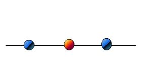
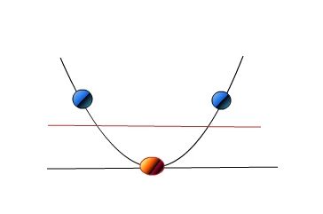
视觉化演示
2.1 如何利用非线性映射把原始数据转化到高维中?
3维输入向量:
转化到6维空间 Z 中去:
新的决策超平面:
其中W和Z是向量,这个超平面是线性的解出W和b之后,并且带入回原方程:
思考问题:
1: 如何选择合理的非线性转化把数据转到高纬度中?
2: 如何解决计算内积时算法复杂度非常高的问题?
-
核方法(kernel trick)
动机: 在线性SVM中转化为最优化问题时求解的公式计算都是以内积(dot product)的形式出现的

,其中是把训练集中的向量点转化到高维的非线性映射函数,因为内积的算法复杂度非常大,所以我们利用核函数来取代计算非线性映射函数的内积
3.1 以下核函数和非线性映射函数的内积等同
3.2 常用的核函数(kernel functions)
- h度多项式核函数(polynomial kernel of degree h):

-
高斯径向基核函数(Gaussian radial basis function kernel):

- S型核函数(Sigmoid function kernel):

如何选择使用哪个kernel?根据先验知识,比如图像分类,通常使用RBF,文字不使用RBF,尝试不同的kernel,根据结果准确度而定。
3.3 核函数举例:
假设定义两个向量: x = (x1, x2, x3); y = (y1, y2, y3)
定义方程:f(x) = (x1x1, x1x2, x1x3, x2x1, x2x2, x2x3, x3x1, x3x2, x3x3)
K(x, y ) = (
假设x = (1, 2, 3); y = (4, 5, 6).
f(x) = (1, 2, 3, 2, 4, 6, 3, 6, 9)
f(y) = (16, 20, 24, 20, 25, 36, 24, 30, 36)
K(x, y) = (4 + 10 + 18 ) ^2 = 32^2 = 1024
同样的结果,使用kernel方法计算容易很多。
- SVM扩展可解决多个类别分类问题
对于每个类,有一个当前类和其他类的二类分类器(one-vs-rest)
利用SVM进行人脸识别实例:
from __future__ import print_function
# 从time模块导入time,因为有些步骤需要计时
from time import time
# 打印出一些程序进展信息
import logging
# 绘图的包,即最后将我们预测出来的人脸打印出来
import matplotlib.pyplot as plt

from sklearn.cross_validation import train_test_split
from sklearn.datasets import fetch_lfw_people
from sklearn.grid_search import GridSearchCV
from sklearn.metrics import classification_report
from sklearn.metrics import confusion_matrix
from sklearn.decomposition import PCA
from sklearn import svm

# 打印输出日志信息
logging.basicConfig(level=logging.INFO, format='%(asctime)s%(message)s')
# 下载数据集--户外脸部数据集lfw(Labeled Faces in the Wild)
# minfaces_per_person:int,可选默认无,提取的数据集仅保留包含min_faces_per_person不同图片的人的照片
# resize调整每张人脸图片的比例,默认是0.5
lfw_people = fetch_lfw_people(min_faces_per_person=70, resize=0.4)
# 返回数据集有多少个实例,h是多少,w是多少
n_samples, h, w = lfw_people.images.shape
# X矩阵用来装特征向量,得到数据集的所有实例
# 每一行是一个实例,每一列是个特征值
X = lfw_people.data
# X矩阵调用shape返回矩阵的行数和列数,
# X.shape[1]返回矩阵的列数,对应的特征向量的维度或者特征点多少
n_features = X.shape[1]
# 获取特征结果集,提取每个实例对应的每个人脸
# y为classlabel目标分类标记,即不同人的身份
y = lfw_people.target
# 数据集中有多少个人,以人名组成列表返回
target_names = lfw_people.target_names
# shape[0]就是多少行,多少个人,多少类
n_classes = target_names.shape[0]

print("Total dataset size:")  # 数据集中信息
print("n_samples:%d" % n_samples)  # 数据个数1288
print("n_features:%d" % n_features)  # 特征个数,维度1850
print("n_classes:%d" % n_classes)  # 结果集类别个数,即多少个人

# 结果
# Total dataset size:
# n_samples:1288
# n_features:1850
# n_classes:7

# 利用train_test_split拆分训练集合测试集
# test_size=0.25表示随机抽取25%的测试集
X_train, X_test, y_train, y_test = train_test_split(X, y, test_size=0.25)

# 采用PCA降维,原始数据的特征向量维度非常高,意味着训练模型的复杂度非常高
# 保存的组件数目,也即保留下来的特征个数n
n_components = 150

print("Exreacting the top %d eigenfaces from %faces" % (n_components, X_train.shape[0]))
# 初始时间
t0 = time()
# 降维
pca = PCA(n_components=n_components, whiten=True).fit(X_train)
print("pca done in %0.3fs" % (time() - t0))
# 从人脸中提取特征点,对于人脸的一张照片提取的特征值名为eigenfaces
eigenfaces = pca.components_.reshape((n_components, h, w))

print("projecting the input data on the eigenfaces orthonormal basis")
t0 = time()
# 把训练集特征向量转化为更低维的矩阵
X_train_pca = pca.transform(X_train)
# 把测试集的特征向量转化为更低维的矩阵
X_test_pca = pca.transform(X_test)
print("done in %0.3fs" % (time() - t0))

# 训练一个支持向量机的分类model——构造分类器
print("Fitting the classifier to the training set")
t0 = time()

# c是一个对错误德部分的惩罚
# gamma的参数对不同核函数有不同的表现,gamma表示使用多少比例的特征点
# 使用不同的c和不同值的gamma,进行多个量的尝试,然后进行搜索,选出准确率最高模型
param_grid = {
    'C': [1e3, 5e3, 1e4, 5e4, 1e5],
    'gamma': [0.0001, 0.0005, 0.001, 0.005, 0.01, 0.1]
}
# 调用SVM进行分类搜索哪对组合产生最好的归类精确度
# ernel:rbf高斯径向基核函数   class_weight权重
# 把所有我们所列参数的组合都放在SVC里面进行计算,最后看出哪一组函数的表现度最好
clf = GridSearchCV(svm.SVC(kernel='rbf', class_weight='balanced'), param_grid=param_grid)
clf = clf.fit(X_train_pca, y_train)
print("fit done in %0.3fs" % (time() - t0))
print("Best estimator found by grid search:")
print(clf.best_estimator_)

##################进行评估准确率计算######################
print("Predicting people's names on the test set")
t0 = time()
# 预测新的分类
y_pred = clf.predict(X_test_pca)
print("done in %0.3fs" % (time() - t0))
# 通过classification_report方法进行查看,可以得到预测结果中哪些是正确
print(classification_report(y_test, y_pred, target_names=target_names))
# confusion_matrix是建一个n*n的方格,横行和纵行分别表示真实的每一组测试的标记和测试集标记的差别
# 对角线表示的是正确的值,对角线数字越多表示准确率越高
print(confusion_matrix(y_test, y_pred, labels=range(n_classes)))


# 将测试标记过进行展示,即先弄一个通用的图片可视化函数:
def plot_gallery(images, titles, h, w, n_row=3, n_col=4):
    """Helper function to plot a gallery of portraits"""
    # 建立图作为背景
    # 自定义画布大小
    plt.figure(figsize=(1.8 * n_col, 2.4 * n_row))
    # 位置调整
    plt.subplots_adjust(bottom=0, left=.01, right=.99, top=.90, hspace=.35)
    for i in range(n_row * n_col):
        # 设置画布划分以及图像在画布上输出的位置
        plt.subplot(n_row, n_col, i + 1)
        # 在轴上显示图片
        plt.imshow(images[i].reshape((h, w)), cmap=plt.cm.gray)
        # 整个画板的标题
        plt.title(titles[i], size=12)
        # 获取或设置x、y轴的当前刻度位置和标签
        plt.xticks(())
        plt.yticks(())


# 预测函数归类标签和实际归类标签打印
# 返回预测人脸姓和测试人脸姓的对比title
def title(y_pred, y_test, target_names, i):
    # rsplit(' ',1)从右边开始以右边第一个空格为界,分成两个字符
    # 组成一个list
    # 此处代表把'姓'和'名'分开,然后把后面的姓提出来
    # 末尾加[-1]代表引用分割后的列表最后一个元素
    pred_name = target_names[y_pred[i]].rsplit(' ', 1)[-1]
    true_name = target_names[y_test[i]].rsplit(' ', 1)[-1]
    return 'predicted:%s\ntrue:  %s' % (pred_name, true_name)


# 预测出的人名
prediction_titles = [title(y_pred, y_test, target_names, i)
                     for i in range(y_pred.shape[0])]
# 测试集的特征向量矩阵和要预测的人名打印
plot_gallery(X_test, prediction_titles, h, w)
# 打印原图和预测的信息
eigenface_titles = ["eigenface %d" % i for i in range(eigenfaces.shape[0])]
# 调用plot_gallery函数打印出实际是谁,预测的谁,以及提取过特征的脸
# plot_gallery(eigenfaces, eigenface_titles, h, w)

plt.show()

# 结果
# Predicting people's names on the test set
# done in 0.053s
#                    precision    recall  f1-score   support
#      Ariel Sharon       0.89      0.47      0.62        17
#      Colin Powell       0.77      0.93      0.84        60
#   Donald Rumsfeld       0.94      0.64      0.76        25
#     George W Bush       0.83      0.96      0.89       137
# Gerhard Schroeder       0.88      0.79      0.83        28
#       Hugo Chavez       1.00      0.47      0.64        15
#        Tony Blair       0.91      0.78      0.84        40
#       avg / total       0.85      0.84      0.83       322
# [[  8   5   0   4   0   0   0]
#  [  0  56   0   4   0   0   0]
#  [  0   2  16   7   0   0   0]
#  [  0   6   0 131   0   0   0]
#  [  1   1   0   2  22   0   2]
#  [  0   1   0   5   1   7   1]
#  [  0   2   1   4   2   0  31]]
结果:

