两万字总结python之pandas库
为什么要学习pandas?
那么问题来了:
numpy已经能够帮助我们处理数据,能够结合matplotlib解决我们数据分析的问题,那么pandas学习的目的在什么地方呢?
numpy能够帮我们处理处理数值型数据,但是这还不够, 很多时候,我们的数据除了数值之外,还有字符串,还有时间序列等。
比如:我们通过爬虫获取到了存储在数据库中的数据
所以,pandas出现了。
什么是Pandas?
Pandas的名称来自于面板数据(panel data)
Pandas是一个强大的分析结构化数据的工具集,基于NumPy构建,提供了高级数据结构和数据操作工具,它是使Python成为强大而高效的数据分析环境的重要因素之一。
-
一个强大的分析和操作大型结构化数据集所需的工具集
-
基础是NumPy,提供了高性能矩阵的运算
-
提供了大量能够快速便捷地处理数据的函数和方法
-
应用于数据挖掘,数据分析
-
提供数据清洗功能
Pandas的数据结构:
import pandas as pd
Pandas有两个最主要也是最重要的数据结构: Series和DataFrame
官网:
http://pandas.pydata.org/
目录
-
Series介绍及其基本操作
-
DateFrame介绍及其基本操作
-
Pandas的索引操作详细介绍
-
Pandas的对齐运算
-
Pandas的函数应用
-
层级索引(hierarchical indexing)
-
Pandas统计计算和描述
Series
Series是一种一维标记的数组型对象,能够保存任何数据类型(int, str, float, python object…),包含了数据标签,称为索引。
- 类似一维数组的对象,index =['名字,‘年龄’,‘班级’]
- 由数据和索引组成
- 索引(index)在左,数据(values)在右
- 索引是自动创建的(也可以自己指定)

Series创建
- 通过list创建
import pandas as pd
import numpy as np
# 2.1 通过list创建
s1 = pd.Series([1,2,3,4,5])
s1
结果:
0    1
1    2
2    3
3    4
4    5
dtype: int64
- 通过数组创建
# 2.2 通过数组创建
arr1 = np.arange(1,6)
print(arr1)
s2 = pd.Series(arr1)
s2
结果:
[1 2 3 4 5]
0    1
1    2
2    3
3    4
4    5
dtype: int32
指定索引名称:
#索引长度和数据长度必须相同。
s2 = pd.Series(arr1,index=['a','b','c','d','e'])
s2
结果:
a    1
b    2
c    3
d    4
e    5
dtype: int32
属性index和values
print(s1.values)
print('='*30)
print(s1.index)
[1 2 3 4 5]
==============================
RangeIndex(start=0, stop=5, step=1)
- 通过字典创建
# 2.3 通过字典创建
dict = {
     'name':'李宁','age':18,'class':'三班'}
s3 = pd.Series(dict,index = ['name','age','class','sex'])
s3
结果:
name      李宁
age       18
class     三班
sex      NaN
dtype: object
Series的基本用法
- isnull 和 notnull 检查缺失值
# isnull 和 notnull 检查缺失值
print(s3.isnull())  #判断是否为空  空就是True
print('='*30)
print(s3.notnull()) #判断是否不为空  非空True
结果:
name     False
age      False
class    False
sex       True
dtype: bool
==============================
name      True
age       True
class     True
sex      False
dtype: bool
- 通过索引获取数据
print(s3)
print('='*30)
# 下标
print(s3[0])
print('='*30)
# 标签名
print(s3['age'])
print('='*30)
# 选取多个
print(s3[['name','age']])  # s3[[1,3]]
print('='*30)
# 切片
print(s3[1:3])
print('='*30)
print(s3['name':'class'])   #标签切片 包含末端数据
print('='*30)
#布尔索引
print(s2[s2>3])
结果:
name      李宁
age       18
class     三班
sex      NaN
dtype: object
==============================
李宁
==============================
18
==============================
name    李宁
age     18
dtype: object
==============================
age      18
class    三班
dtype: object
==============================
name     李宁
age      18
class    三班
dtype: object
==============================
3    4
4    5
dtype: int32
- 索引与数据的对应关系不被运算结果影响
#索引与数据的对应关系不被运算结果影响
print(s2+2)
print('='*30)
print(s2>2)
结果:
0    3
1    4
2    5
3    6
4    7
dtype: int32
==============================
0    False
1    False
2     True
3     True
4     True
dtype: bool
- name属性
s2.name = 'temp'  #对象名
s2.index.name = 'year'  #对象的索引名
s2
结果:
year
a    1
b    2
c    3
d    4
e    5
Name: temp, dtype: int32
- head和tail方法
print(s2.head(3))  #无参数默认前5行
print('='*30)
print(s2.tail(2))  #无参数尾部默认后5行
结果:
0    1
1    2
2    3
dtype: int32
==============================
3    4
4    5
dtype: int32
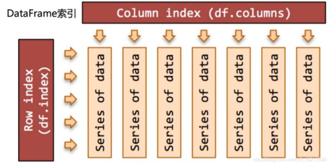
DateFrame
DataFrame是一个表格型的数据结构,它含有一组有序的列,每列可以是不同类型的值。DataFrame既有行索引也有列索引,它可以被看做是由Series组成的字典(共用同一个索引),数据是以二维结构存放的。
- 类似多维数组/表格数据(如,excel,R中的data.frame)
- 每列数据可以是不同的类型
- 索引包括列索引和行索引

DateFrame构建
字典类:
-
数组、列表或元组构成的字典构造dataframe
-
Series构成的字典构造dataframe
-
字典构成的字典构造dataframe
列表类:
-
2D ndarray 构造dataframe
-
字典构成的列表构造dataframe
-
Series构成的列表构造dataframe
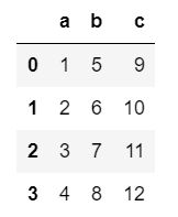
数组、列表或元组构成的字典构造dataframe
import numpy as np
import pandas as pd
# 数组、列表或元组构成的字典构造dataframe
#构造一个字典
data = {
     'a':[1,2,3,4],
        'b':(5,6,7,8),
       'c':np.arange(9,13)}
#构造dataframe
frame = pd.DataFrame(data)
frame
结果:
一些属性操作:
#index属性查看行索引
print(frame.index)
print('='*30)
#columns属性查看列索引
print(frame.columns)
print('='*30)
#values属性查看值
print(frame.values)
print('='*30)
#指定index
frame = pd.DataFrame(data,index=['A','B','C','D'])
print(frame)
print('='*30)
#指定列索引
frame = pd.DataFrame(data,index=['A','B','C','D'],columns=['a','b','c','d'])#若指定多余的列,则那一列值为NAN
print(frame)
结果:
RangeIndex(start=0, stop=4, step=1)
==============================
Index(['a', 'b', 'c'], dtype='object')
==============================
[[ 1  5  9]
 [ 2  6 10]
 [ 3  7 11]
 [ 4  8 12]]
==============================
   a  b   c
A  1  5   9
B  2  6  10
C  3  7  11
D  4  8  12
==============================
   a  b   c    d
A  1  5   9  NaN
B  2  6  10  NaN
C  3  7  11  NaN
D  4  8  12  NaN
Series构成的字典构造dataframe
#2.Series构成的字典构造dataframe
pd1 = pd.DataFrame({
     'a':pd.Series(np.arange(3)),
                   'b':pd.Series(np.arange(3,5))})
print(pd1)
结果:
   a    b
0  0  3.0
1  1  4.0
2  2  NaN
字典构成的字典构造dataframe
#3.字典构成的字典构造dataframe
#字典嵌套
data1 = {

    'a':{
     'apple':3.6,'banana':5.6},
    'b':{
     'apple':3,'banana':5},
    'c':{
     'apple':3.2}
}
pd2 = pd.DataFrame(data1)
print(pd2)
结果:
   a  b    c
apple   3.6  3  3.2
banana  5.6  5  NaN
2D ndarray 构造dataframe
#构造二维数组对象
arr1 = np.arange(12).reshape(4,3)

frame1 = pd.DataFrame(arr1)
print(frame1)
结果:
 0   1   2
0  0   1   2
1  3   4   5
2  6   7   8
3  9  10  11
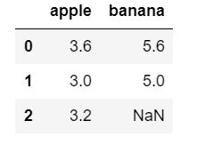
字典构成的列表构造dataframe
l1 = [{
     'apple':3.6,'banana':5.6},{
     'apple':3,'banana':5},{
     'apple':3.2}]
pd3 = pd.DataFrame(l1)
pd3
结果:
Series构成的列表构造dataframe
l2 = [pd.Series(np.random.rand(3)),pd.Series(np.random.rand(2))]
pd4 = pd.DataFrame(l2)
print(pd4)
结果:
          0         1         2
0  0.479686  0.107307  0.908551
1  0.032230  0.626875       NaN
DataFrame的基本用法
- T转置
- 通过列索引获取列数据(Series类型)
- 增加列数据
- 删除列
T转置
#dataframe
pd5 = pd.DataFrame(np.arange(9).reshape(3,3),index=['a','c','b'],columns=['A','B','C'])
print(pd5)
结果:
A  B  C
a  0  1  2
c  3  4  5
b  6  7  8
#和numpy一样 进行转置   行与列进行转置
print(pd5.T)
结果:
  a  c  b
A  0  3  6
B  1  4  7
C  2  5  8
通过列索引获取列数据(Series类型)
pd5['A']
print(type(pd5['A']))
结果:
<class 'pandas.core.series.Series'>
增加列数据
pd5['D'] = [1,2,3]
print(pd5)
结果:
 A  B  C  D
a  0  1  2  1
c  3  4  5  2
b  6  7  8  3
删除列
del(pd5['D'])
print(pd5)
结果:
A  B  C
a  0  1  2
c  3  4  5
b  6  7  8
Pandas的索引操作
索引对象Index
1. Series和DataFrame中的索引都是Index对象
代码举例:
import numpy as np
import pandas as pd
ps1 = pd.Series(range(5),index=['a','b','c','d','e'])
print(type(ps1.index))
print('='*30)
pd1 = pd.DataFrame(np.arange(9).reshape(3,3),index = ['a','b','c'],columns = ['A','B','C'])
print(type(pd1.index))
结果:
<class 'pandas.core.indexes.base.Index'>
==============================
<class 'pandas.core.indexes.base.Index'>
2. 索引对象不可变,保证了数据的安全
代码举例:
pd1.index[1] = 2
pd1
结果:
TypeError                                 Traceback (most recent call last)
<ipython-input-16-8d21a7039bc5> in <module>()
----> 1 pd1.index[1] = 2

D:\Anaconda\lib\site-packages\pandas\core\indexes\base.py in __setitem__(self, key, value)
   1668
   1669     def __setitem__(self, key, value):
-> 1670         raise TypeError("Index does not support mutable operations")
   1671
   1672     def __getitem__(self, key):

TypeError: Index does not support mutable operations
常见的Index种类
- Index,索引
- Int64Index,整数索引
- MultiIndex,层级索引
- DatetimeIndex,时间戳类型
Series索引
- index 指定行索引名
ser_obj = pd.Series(range(5), index = ['a', 'b', 'c', 'd', 'e'])
print(ser_obj.head())
结果:
a    0
b    1
c    2
d    3
e    4
dtype: int64
- 行索引
ser_obj[‘label’]
ser_obj[pos]
# 行索引
print(ser_obj['b'])
print(ser_obj[2])
结果:
1
2
- 切片索引
ser_obj[2:4]
ser_obj[‘label1’: ’label3’]
注意,按索引名切片操作时,是包含终止索引的。
代码举例:
# 切片索引
print(ser_obj[1:3])
print(ser_obj['b':'d'])
结果:
b    1
c    2
dtype: int64
b    1
c    2
d    3
dtype: int64
- 不连续索引
ser_obj[[‘label1’, ’label2’, ‘label3’]]
ser_obj[[0,1,2]]
代码举例:
# 不连续索引
print(ser_obj[[0, 2, 4]])
print(ser_obj[['a', 'e']])
结果:
a    0
c    2
e    4
dtype: int64
a    0
e    4
dtype: int64
- 布尔索引
# 布尔索引
ser_bool = ser_obj > 2
print(ser_bool)
print(ser_obj[ser_bool])

print(ser_obj[ser_obj > 2])
结果:
a    False
b    False
c    False
d     True
e     True
dtype: bool
d    3
e    4
dtype: int64
d    3
e    4
dtype: int64
DataFrame索引
-
columns 指定列索引名
import numpy as np

df_obj = pd.DataFrame(np.random.randn(5,4), columns = ['a', 'b', 'c', 'd'])
print(df_obj.head())
结果:
 a         b         c         d
0 -0.241678  0.621589  0.843546 -0.383105
1 -0.526918 -0.485325  1.124420 -0.653144
2 -1.074163  0.939324 -0.309822 -0.209149
3 -0.716816  1.844654 -2.123637 -1.323484
4  0.368212 -0.910324  0.064703  0.486016
- 列索引
df_obj[[‘label’]]
示例代码:
# 列索引
print(df_obj['a']) # 返回Series类型
结果:
0   -0.241678
1   -0.526918
2   -1.074163
3   -0.716816
4    0.368212
Name: a, dtype: float64
- 不连续索引
df_obj[[‘label1’, ‘label2’]]
代码举例:
# 不连续索引
print(df_obj[['a','c']])
结果:
       a         c
0 -0.241678  0.843546
1 -0.526918  1.124420
2 -1.074163 -0.309822
3 -0.716816 -2.123637
4  0.368212  0.064703
高级索引:标签、位置和混合(不建议使用,不再展开讨论)
Pandas的高级索引有3种
1. loc 标签索引
DataFrame 不能直接切片,可以通过loc来做切片
loc是基于标签名的索引,也就是我们自定义的索引名
代码举例:
# 标签索引 loc
# Series
print(ser_obj['b':'d'])
print(ser_obj.loc['b':'d'])

# DataFrame
print(df_obj['a'])

# 第一个参数索引行,第二个参数是列
print(df_obj.loc[0:2, 'a'])
结果:
b    1
c    2
d    3
dtype: int64
b    1
c    2
d    3
dtype: int64

0   -0.241678
1   -0.526918
2   -1.074163
3   -0.716816
4    0.368212
Name: a, dtype: float64
0   -0.241678
1   -0.526918
2   -1.074163
Name: a, dtype: float64
2.位置索引
作用和loc一样,不过是基于索引编号来索引
示例代码:
# 整型位置索引 iloc
# Series
print(ser_obj[1:3])
print(ser_obj.iloc[1:3])

# DataFrame
print(df_obj.iloc[0:2, 0]) # 注意和df_obj.loc[0:2, 'a']的区别,包括不包括的问题
结果:
b    1
c    2
dtype: int64
b    1
c    2
dtype: int64

0   -0.241678
1   -0.526918
Name: a, dtype: float64
注意:
标签的切片索引是包含末尾位置的
索引的一些基本操作
-
重建索引
-
增
-
删
-
改
-
查
import numpy as np
import pandas as pd
ps1 = pd.Series(range(5),index=[‘a’,‘b’,‘c’,‘d’,‘e’])
print(ps1)
print(’=’*30)
pd1 = pd.DataFrame(np.arange(9).reshape(3,3),index = [‘a’,‘b’,‘c’],columns = [‘A’,‘B’,‘C’])
print(pd1)
结果:
a 0
b 1
c 2
d 3
e 4
dtype: int64
==============================
A B C
a 0 1 2
b 3 4 5
c 6 7 8
1.重建索引
对于Series
#1.reindex 创建一个符合新索引的新对象
ps2 = ps1.reindex(['a','b','c','d','e','f'])#必须是原本有的加上没有的列名
ps2
结果:
a    0.0
b    1.0
c    2.0
d    3.0
e    4.0
f    NaN
dtype: float64
对于dataframe
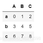
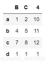
#行索引重建
pd2 = pd1.reindex(['a','b','c','d'])
pd2
结果:

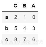
#列索引重建
pd3 = pd1.reindex(columns = ['C','B','A'])
pd3
结果:
2.增
对于series
ps1
结果:
a    0
b    1
c    2
d    3
e    4
dtype: int32
ps1['g'] = 9
ps1
结果:
a    0
b    1
c    2
d    3
e    4
g    9
dtype: int64
若不想直接操作原对象:
s1 = pd.Series({
     'f':999})
ps3 = ps1.append(s1)
ps3
结果:
a      0
b      1
c      2
d      3
e      4
g      9
f    999
dtype: int64
对于dataframe
pd1
结果:
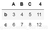
#增加列
pd1[4] = [10,11,12]
pd1
结果:

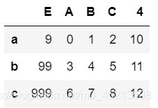
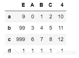
# 插入
pd1.insert(0,'E',[9,99,999])#在第1列插入
pd1
结果:
增加行
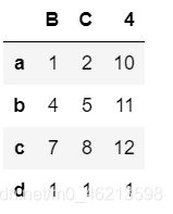
#标签索引loc
pd1.loc['d'] = [1,1,1,1,1]
pd1
结果:
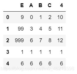
row = {
     'E':6,'A':6,'B':6,'C':6,4:6}
pd5 = pd1.append(row,ignore_index=True)
#ignore_index 参数默认值为False,如果为True,会对新生成的dataframe使用新的索引(自动产生),忽略原来数据的索引。
pd5
结果:
3.删
对于series
#del
ps1
结果:
a    0
b    1
c    2
d    3
e    4
g    9
dtype: int64
del ps1['b']
ps1
结果:
a    0
c    2
d    3
e    4
g    9
dtype: int64
对于dataframe
pd1
结果:
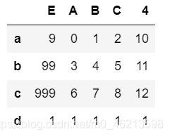
del pd1['E']
pd1
结果:

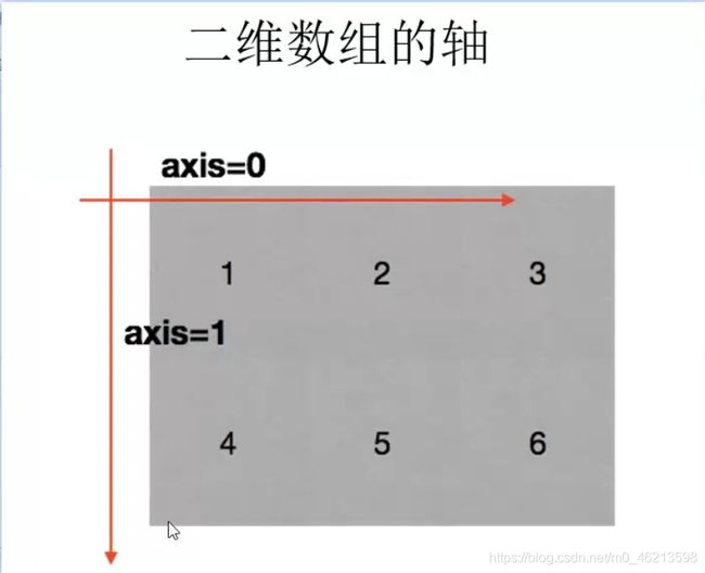
drop函数:删除轴上的数据,默认非原地操作,可通过属性进行修改
#drop  删除轴上数据
#删除一条
ps6 = ps1.drop('g')
ps6
结果:
a    0
c    2
d    3
e    4
dtype: int64
#删除多条
ps1.drop(['c','d'])
结果:
a    0
e    4
g    9
dtype: int64
#dataframe
#删除行
pd1.drop('a')
结果:

pd1.drop(['a','d'])
结果:
#删除列
pd1.drop('A',axis=1)  #1列  0 行
结果:
pd1.drop('A',axis='columns')
结果:
#inplace属性   在原对象上删除,并不会返回新的对象
ps1
结果:
a    0
c    2
d    3
e    4
g    9
dtype: int64
ps1.drop('d',inplace=True)
ps1
结果:
a    0
c    2
e    4
g    9
dtype: int64
4.改
ps1 = pd.Series(range(5),index=['a','b','c','d','e'])
print(type(ps1.index))
ps1
结果:
<class 'pandas.core.indexes.base.Index'>
a    0
b    1
c    2
d    3
e    4
dtype: int32
pd1 = pd.DataFrame(np.arange(9).reshape(3,3),index = ['a','b','c'],columns = ['A','B','C'])
pd1
结果:

ps1['a'] = 999
ps1
结果:
a    999
b      1
c      2
d      3
e      4
dtype: int32
ps1[0] = 888
ps1
结果:
a    888
b      1
c      2
d      3
e      4
dtype: int32
对于dataframe操作:
#直接使用索引
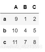
pd1['A'] = [9,10,11]
pd1
结果:
# 变成增加列的操作
pd1['a'] = 777
pd1
结果:

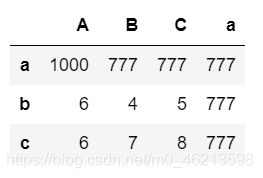
#loc 标签索引
pd1.loc['a'] =777#增加索引为a的这一行
pd1

pd1.loc['a','A'] = 1000#修改单个值
pd1
结果:
5.查
对于series
#Series
# 1.行索引
ps1
结果:
a    888
b      1
c      2
d      3
e      4
dtype: int32
print(ps1['a'])
print('='*30)
print(ps1[0])
结果:
888
==============================
888
…请参考series基本操作
对于dataframe
pd1
结果:

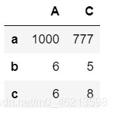
#取多列
pd1[['A','C']]
结果:
#选取一个值
pd1['A']['a']
结果:
1000
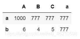
#2.切片
pd1[:2]  #获取行
结果:
…对于截取部分操作请参考loc和iloc
Pandas的对齐运算
是数据清洗的重要过程,可以按索引对齐进行运算,如果没对齐的位置则补NaN,最后也可以填充NaN
import numpy as np
import pandas as pd
1.算术运算符对其
对于series
#Series
s1 = pd.Series(np.arange(4),index = ['a','b','c','d'])
s2 = pd.Series(np.arange(5),index = ['a','c','e','f','g'])
print(s1)
print('='*30)
print(s2)
结果:
a    0
b    1
c    2
d    3
dtype: int32
==============================
a    0
c    1
e    2
f    3
g    4
dtype: int32
print(s1+s2)
结果:
a    0.0
b    NaN
c    3.0
d    NaN
e    NaN
f    NaN
g    NaN
dtype: float64
对于DataFrame
#DataFrame
df1 = pd.DataFrame(np.arange(12).reshape(4,3),index = ['a','b','c','d'],columns= list('ABC'))
df2 = pd.DataFrame(np.arange(9).reshape(3,3),index = ['a','d','f'],columns= list('ABD'))
print(df1)
print('='*30)
print(df2)
print('='*30)
print(df1+df2)
结果:
 A   B   C
a  0   1   2
b  3   4   5
c  6   7   8
d  9  10  11
==============================
   A  B  D
a  0  1  2
d  3  4  5
f  6  7  8
==============================
      A     B   C   D
a   0.0   2.0 NaN NaN
b   NaN   NaN NaN NaN
c   NaN   NaN NaN NaN
d  12.0  14.0 NaN NaN
f   NaN   NaN NaN NaN
2.使用填充值的算术方法
s1.add(s2,fill_value =0 )
结果:
a    0.0
b    1.0
c    3.0
d    3.0
e    2.0
f    3.0
g    4.0
dtype: float64
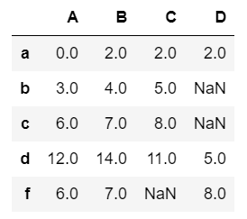
df1.add(df2,fill_value = 0)
结果:
对于二维的来说,两个不存在的值相加还是NaN
df1.rdiv(1) #字母r开头 会翻转参数,等价于1/df1
结果:

3.DataFrame和Series混合运算(广播机制)
对于series
arr = np.arange(12).reshape(3,4)
arr
结果:
array([[ 0,  1,  2,  3],
       [ 4,  5,  6,  7],
       [ 8,  9, 10, 11]])
arr[0]
结果:
array([0, 1, 2, 3])
arr-arr[0]
结果:
array([[0, 0, 0, 0],
       [4, 4, 4, 4],
       [8, 8, 8, 8]])
对于df
df1
结果:

s4 = df1['A']
s4
结果:
a    0
b    3
c    6
d    9
Name: A, dtype: int32
df1.sub(s4,axis=0) # == axis=0
结果:
Pandas的函数应用
apply 和 applymap
1. 可直接使用NumPy的函数
示例代码:
# Numpy ufunc 函数
df = pd.DataFrame(np.random.randn(5,4) - 1)
print(df)

print(np.abs(df))
运行结果:
   0         1         2         3
0 -0.062413  0.844813 -1.853721 -1.980717
1 -0.539628 -1.975173 -0.856597 -2.612406
2 -1.277081 -1.088457 -0.152189  0.530325
3 -1.356578 -1.996441  0.368822 -2.211478
4 -0.562777  0.518648 -2.007223  0.059411

          0         1         2         3
0  0.062413  0.844813  1.853721  1.980717
1  0.539628  1.975173  0.856597  2.612406
2  1.277081  1.088457  0.152189  0.530325
3  1.356578  1.996441  0.368822  2.211478
4  0.562777  0.518648  2.007223  0.059411
2. 通过apply将函数应用到列或行上
示例代码:
# 使用apply应用行或列数据
#f = lambda x : x.max()
print(df.apply(lambda x : x.max()))
结果:
0   -0.062413
1    0.844813
2    0.368822
3    0.530325
dtype: float64
注意指定轴的方向,默认axis=0,方向是列
示例代码:
# 指定轴方向,axis=1,方向是行
print(df.apply(lambda x : x.max(), axis=1))
结果:
0    0.844813
1   -0.539628
2    0.530325
3    0.368822
4    0.518648
dtype: float64
3. 通过applymap将函数应用到每个数据上
示例代码:
# 使用applymap应用到每个数据
f2 = lambda x : '%.2f' % x
print(df.applymap(f2))
结果:
   0      1      2      3
0  -0.06   0.84  -1.85  -1.98
1  -0.54  -1.98  -0.86  -2.61
2  -1.28  -1.09  -0.15   0.53
3  -1.36  -2.00   0.37  -2.21
4  -0.56   0.52  -2.01   0.06
排序
1. 索引排序
sort_index()
排序默认使用升序排序,ascending=False 为降序排序
对于series
s1 = pd.Series(np.arange(4),index=list('dbca'))
s1
结果:
d    0
b    1
c    2
a    3
dtype: int32
s1.sort_index() #默认升序
结果:
a    3
b    1
c    2
d    0
dtype: int32
s1.sort_index(ascending = False) #降序
结果:
d    0
c    2
b    1
a    3
dtype: int32
对于dataframe
pd1 = pd.DataFrame(np.arange(12).reshape(4,3),index=list('bdca'),columns = list('BCA'))
pd1
结果:
B	C	A
b	0	1	2
d	3	4	5
c	6	7	8
a	9	10	11
#按照行排序
pd1.sort_index()
结果:
B	C	A
a	9	10	11
b	0	1	2
c	6	7	8
d	3	4	5
#按照列排序
pd1.sort_index(axis=1)
结果:
A	B	C
b	2	0	1
d	5	3	4
c	8	6	7
a	11	9	10
2.按值排序
sort_values(by=‘column name’)
根据某个唯一的列名进行排序,如果有其他相同列名则报错。
对于series
s1['a'] = np.nan
s1
结果:
d    0.0
b    1.0
c    2.0
a    NaN
dtype: float64
s1.sort_values() #根据值的大小进行排序,当有缺失值,会默认排最后
结果:
d    0.0
b    1.0
c    2.0
a    NaN
dtype: float64
对于dataframe
pd1
结果:
	B	C	A
b	0	1	2
d	3	4	5
c	6	7	8
a	9	10	11
pd1.sort_values(by=['A','B'],ascending=False)#指定多列排序
结果:
	B	C	A
a	9	10	11
c	6	7	8
d	3	4	5
b	0	1	2
pd2.sort_values(by='b') #指定b列排序
结果:
	a	b	c
1	7	-1	6
0	3	1	0
2	9	4	-3
3	0	8	2
3.唯一值和成员属性
s1 = pd.Series([2,6,8,9,8,3,6],index=['a','a','c','c','c','c','c'])
s1
结果:
a    2
a    6
c    8
c    9
c    8
c    3
c    6
dtype: int64
#返回一个series中的唯一值
s2=s1.unique()   #返回一个数组
s2
结果:
array([2, 6, 8, 9, 3], dtype=int64)
s1 = pd.Series([2,6,8,9,8,3,6])
s1
结果:
0    2
1    6
2    8
3    9
4    8
5    3
6    6
dtype: int64
#判断多个值是否存在
s1.isin([8,2])
结果:
0     True
1    False
2     True
3    False
4     True
5    False
6    False
dtype: bool
4.处理缺失数据
示例代码:
df_data = pd.DataFrame([np.random.randn(3), [1., 2., np.nan],
                       [np.nan, 4., np.nan], [1., 2., 3.]])
print(df_data.head())
结果:
         0         1         2
0 -0.281885 -0.786572  0.487126
1  1.000000  2.000000       NaN
2       NaN  4.000000       NaN
3  1.000000  2.000000  3.000000
1. 判断是否存在缺失值:isnull()
示例代码:
# isnull
print(df_data.isnull())
结果:
   0      1      2
0  False  False  False
1  False  False   True
2   True  False   True
3  False  False  False
2. 丢弃缺失数据:dropna()
根据axis轴方向,丢弃包含NaN的行或列。 示例代码:
# dropna
print(df_data.dropna())

print(df_data.dropna(axis=1))
结果:
   0         1         2
0 -0.281885 -0.786572  0.487126
3  1.000000  2.000000  3.000000

          1
0 -0.786572
1  2.000000
2  4.000000
3  2.000000
3.填充缺失数据:fillna()
示例代码:
# fillna
print(df_data.fillna(-100.))
结果:
     0         1           2
0   -0.281885 -0.786572    0.487126
1    1.000000  2.000000 -100.000000
2 -100.000000  4.000000 -100.000000
3    1.000000  2.000000    3.000000
层级索引(hierarchical indexing)
下面创建一个Series,
在输入索引Index时,输入了由两个子list组成的list,第一个子list是外层索引,第二个list是内层索引。
示例代码:
import pandas as pd
import numpy as np

ser_obj = pd.Series(np.random.randn(12),index=[
                ['a', 'a', 'a', 'b', 'b', 'b', 'c', 'c', 'c', 'd', 'd', 'd'],
                [0, 1, 2, 0, 1, 2, 0, 1, 2, 0, 1, 2]
            ])
print(ser_obj)
结果:
a  0    0.099174
   1   -0.310414
   2   -0.558047
b  0    1.742445
   1    1.152924
   2   -0.725332
c  0   -0.150638
   1    0.251660
   2    0.063387
d  0    1.080605
   1    0.567547
   2   -0.154148
dtype: float64
MultiIndex索引对象
打印这个Series的索引类型,显示是MultiIndex
直接将索引打印出来,可以看到有lavels,和labels两个信息。levels表示两个层级中分别有那些标签,labels是每个位置分别是什么标签。
示例代码:
print(type(ser_obj.index))
print(ser_obj.index)
运行结果:
<class 'pandas.indexes.multi.MultiIndex'>
MultiIndex(levels=[['a', 'b', 'c', 'd'], [0, 1, 2]],
           labels=[[0, 0, 0, 1, 1, 1, 2, 2, 2, 3, 3, 3], [0, 1, 2, 0, 1, 2, 0, 1, 2, 0, 1, 2]])
选取子集
根据索引获取数据。因为现在有两层索引,当通过外层索引获取数据的时候,可以直接利用外层索引的标签来获取。
当要通过内层索引获取数据的时候,在list中传入两个元素,前者是表示要选取的外层索引,后者表示要选取的内层索引。
1. 外层选取:
ser_obj[‘outer_label’]
示例代码:
# 外层选取
print(ser_obj['c'])
运行结果:
0   -1.362096
1    1.558091
2   -0.452313
dtype: float64
- 内层选取:
ser_obj[:, ‘inner_label’]
示例代码:
# 内层选取
print(ser_obj[:, 2])
运行结果:
a    0.826662
b    0.015426
c   -0.452313
d   -0.051063
dtype: float64
常用于分组操作、透视表的生成等
交换分层顺序
swaplevel()
swaplevel( )交换内层与外层索引。
示例代码:
print(ser_obj.swaplevel())
运行结果:
0  a    0.099174
1  a   -0.310414
2  a   -0.558047
0  b    1.742445
1  b    1.152924
2  b   -0.725332
0  c   -0.150638
1  c    0.251660
2  c    0.063387
0  d    1.080605
1  d    0.567547
2  d   -0.154148
dtype: float64
交换并排序分层
sortlevel()
.sortlevel( )先对外层索引进行排序,再对内层索引进行排序,默认是升序。
示例代码:
交换并排序分层
print(ser_obj.swaplevel().sortlevel())
运行结果:
0  a    0.099174
   b    1.742445
   c   -0.150638
   d    1.080605
1  a   -0.310414
   b    1.152924
   c    0.251660
   d    0.567547
2  a   -0.558047
   b   -0.725332
   c    0.063387
   d   -0.154148
dtype: float64
Pandas统计计算和描述
示例代码:
arr1 = np.random.rand(4,3)
pd1 = pd.DataFrame(arr1,columns=list('ABC'),index=list('abcd'))
f = lambda x: '%.2f'% x
pd2 = pd1.applymap(f).astype(float)
pd2
运行结果:
      A            B           C
a    0.87        0.26        0.67
b    0.69        0.89        0.17
c    0.94        0.33        0.04
d    0.35        0.46        0.29
常用的统计计算
sum, mean, max, min…
axis=0 按列统计,axis=1按行统计
skipna 排除缺失值, 默认为True
示例代码:
pd2.sum() #默认把这一列的Series计算,所有行求和
pd2.sum(axis='columns') #指定求每一行的所有列的和
pd2.idxmax()#查看每一列所有行的最大值所在的标签索引,同样我们也可以通过axis='columns'求每一行所有列的最大值的标签索引
结果:
A    2.85
B    1.94
C    1.17
dtype: float64


a    1.80
b    1.75
c    1.31
d    1.10
dtype: float64


A    c
B    b
C    a
dtype: object

常用的统计描述
示例代码:
pd2.describe()#查看汇总
运行结果:
                A        B        C
count      4.000000    4.00000        4.000000
mean       0.712500    0.48500        0.292500
std        0.263613    0.28243        0.271585
min        0.350000    0.26000        0.040000
25%        0.605000    0.31250        0.137500
50%        0.780000    0.39500        0.230000
75%        0.887500    0.56750        0.385000
max        0.940000    0.89000        0.670000
#百分比:除以原来的量
pd2.pct_change() #查看行的百分比变化,同样指定axis='columns'列与列的百分比变化
     A                 B                C
a    NaN              NaN             NaN
b    -0.206897        2.423077        -0.746269
c    0.362319        -0.629213        -0.764706
d    -0.627660        0.393939        6.250000
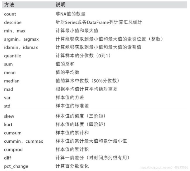
常用的统计描述方法: