Recapping from the previous two posts, this post will utilise machine learning algorithms to predict customers who are mostly likely to purchase caravan policy based on 85 historic socio-demographic and product-ownership data attributes. In the previous post, we talked about using several feature selection methods like forward/backward stepwise selection and lasso regularisation to reduce the number of attributes we should fit into our ML algorithms. We will discuss which set of attributes as identified by different feature selection methods, will give us the best prediction results.
在前两篇文章的基础上,本篇文章将利用机器学习算法,基于85个历史社会人口统计数据和产品所有权数据属性,预测最有可能购买商队政策的客户。 在上一篇文章中,我们讨论了使用一些特征选择方法,例如向前/向后逐步选择和套索正则化,以减少我们应该适合我们的ML算法的属性数量。 我们将讨论通过不同的特征选择方法确定的属性集,这些属性集将为我们提供最佳的预测结果。
Logistic回归模型开发1 (Logistic Regression model development 1)
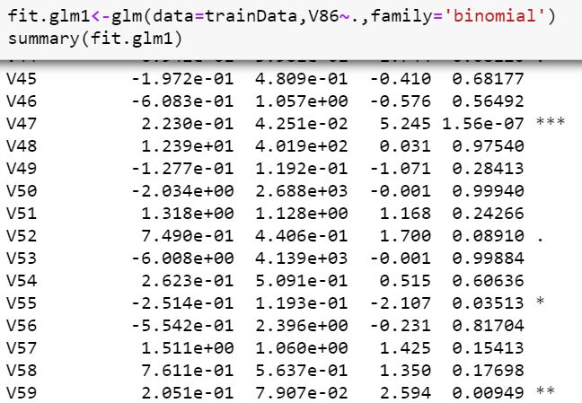
Since the target attribute (i.e. whether the customer purchases or not purchase caravan policy) is binomial discrete, we can use the simplest logistic regression as our first ML algorithm usingglm function from glmnet package. We first fit all the variables in to see how does the model performs using V86~ which means all attributes as the predictor variables other than V86 which is our target variable.
由于目标属性(即客户是否购买房车保单)是二项式离散的,因此我们可以使用最简单的逻辑回归作为第一个使用glmnet包中的glm函数的ML算法。 我们首先拟合所有变量,以查看模型如何使用V86〜执行,这意味着除作为目标变量的V86外,所有属性均作为预测变量。
Observations from this model:
该模型的观察结果:
At 5% significance level, V47 (Contribution car policies), V55 (Contribution life policies), V59 (Contribution fire policies), V76 (Number of life insurances), V82 (Number of boat policies) are significant
在5%的显着性水平下, V47(缴费汽车保单),V55(缴费人寿保单),V59(缴费火险保单),V76(人寿保险数),V82(船保单数)很重要
- Residual deviance is lesser than null deviance which means this model is more useful compared to one without any predictor variables残留偏差小于零偏差,这意味着与没有任何预测变量的模型相比,此模型更有用
Note that the *** signifies the level of significance of this predictor variable.
请注意, ***表示此预测变量的显着性水平。
We can use the Chisq test to check how well is the logistic regression model in comparison with a null model.
我们可以使用Chisq检验来检查逻辑回归模型与null模型相比是否良好。
The p-value is really small which means this model is significantly better than the null model.
p值确实很小,这意味着该模型明显优于空模型。
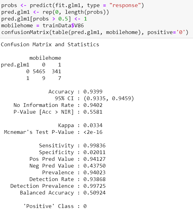
Since our task is to predict if a specific customer will buy caravan policies, we create a confusion matrix by using confusionMatrix function from the caret library to show how many predictions this model has made correctly and incorrectly in our training dataset.
由于我们的任务是预测特定客户是否会购买商队保单,因此我们使用caret库中的confusionMatrix函数创建一个混淆矩阵,以显示该模型在我们的训练数据集中正确或不正确地做出了多少预测。
This model predicted that 9+7=16 customers will buy mobile home policies and 5465+341=5806 will not buy mobile home policies. Of these observations, 5465 out of (5465+9) which is approximately 99.84% (sensitivity) were correctly predicted by the model that these customers will not buy mobile home policies and they indeed not buy it. Whereas, only 7 out of (7+341) which is approximately 2.01% (specificity) were correctly predicted by the model that these customers will buy mobile home policies and they indeed bought it. Hence, this model has high sensitivity but very low specificity.
该模型预测9 + 7 = 16个客户将购买移动房屋保单,而5465 + 341 = 5806将不购买移动房屋保单。 在这些观察结果中,该模型正确地预测了(5465 + 9)中的5465个(灵敏度)约为99.84%(这些敏感性),这些客户不会购买移动房屋保单,而实际上他们也不会购买。 而该模型仅正确地预测了(7 + 341)中的7个(即2.01%)(特异性),这些客户将购买移动房屋保单,而他们确实购买了。 因此,该模型具有高灵敏度但特异性很低。
Note that even though the accuracy of the model is high at 93.99%, it is expected as since our dataset is highly unbalanced with only 348 (6%) of the customers having bought mobile home policies. If we were to predict that all customers will not purchase mobile home policies, we will still get an overall percentage of 5474/5822 of correct predictions which is approximately 94.02% (i.e. No Information Rate). As a result, what we are aiming for in terms of the training error is a model with high specificity since we are trying to identify the customers that will buy mobile home policies.
请注意,尽管该模型的准确性很高,为93.99%,但由于我们的数据集高度失衡,只有348(6%)个购买了移动房屋保单的客户,因此可以预期。 如果我们要预测所有客户都不会购买移动房屋保单,那么我们仍将获得5474/5822正确预测的总百分比,大约为94.02%(即无信息率)。 结果,我们针对训练错误的目标是建立一种具有高度特异性的模型,因为我们试图确定将购买移动房屋保单的客户。
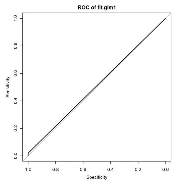
We can illustrate the sensitivity and specificity of the model by plotting a Receiver Operating Characteristic (ROC) curve by using the library pROC.
我们可以通过使用库pROC绘制接收者工作特征(ROC)曲线来说明模型的敏感性和特异性。
What will be ideal in a ROC curve for a good model is for both the sensitivity and specificity to be close to the left top edge of the curve which means area under the curve is 1. However as seen in this plot, the line is far away from the top left edge and area under the curve is only 0.509 which is also obtainable as Balanced Accuracy in the previous Confusion Matrix and Statistics section.
对于一个好的模型,在ROC曲线中理想的是灵敏度和特异性都接近曲线的左上边缘,这意味着曲线下的面积为1。但是,如该图所示,该线很远距左上边缘和曲线下方区域仅0.509,也可以在前面的“混淆矩阵和统计”部分中以“平衡精度”获得。
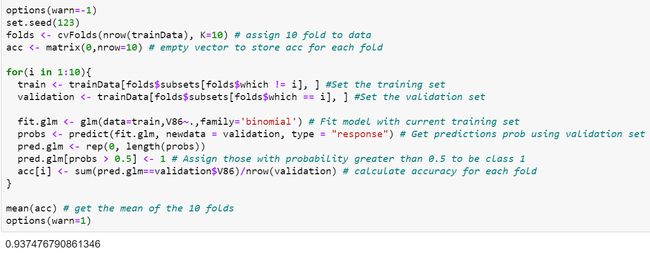
Since we know that our data is highly imbalanced, we can use sampling method like K-Fold Cross Validation approach to get a more accurate value for the accuracy of our model. We will use 10 Fold Cross Validation which involved splitting our training data into 10 folds, and we train 10 models each of them using 9 of the fold as training data and 10th fold as the validation data to get the accuracy of the model. We then obtain the mean of the accuracy of all the 10 models.
由于我们知道我们的数据高度不平衡,因此我们可以使用采样方法(例如K折交叉验证方法)来获得更准确的模型值。 我们将使用10折交叉验证,这涉及将训练数据分成10折,我们使用9折作为训练数据,将10折作为验证数据来训练10个模型,以获取模型的准确性。 然后,我们获得所有10个模型的准确性的平均值。
With 10-Fold Cross Validation, we noted the accuracy of this model is 0.9375.
通过10倍交叉验证,我们注意到该模型的准确性为0.9375。
Logistic回归模型开发2 (Logistic Regression model development 2)
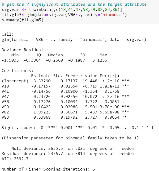
We repeat the above using the set of attributes identified by Forward stepwise selection, Backward stepwise selection and Lasso Regularisation. From there, it can be shown that Lasso Regularisation identified attributes performed better in terms of specificity. Now, we can try to fit another model using 7 significant attributes as identified by the logistic regression trained with Lasso regularisation identified attributes.
我们使用由正向逐步选择,向后逐步选择和套索正则化标识的属性集重复上述操作。 从那里可以看出,在特异性方面,套索正则化确定的属性表现更好。 现在,我们可以尝试使用7个重要属性来拟合另一个模型,该属性由通过套索正则化确定的属性训练的逻辑回归确定。
Observations from this model:
该模型的观察结果:
At 5% significance level, V18 (Lower level education), V47 (Contribution car policies), V59 (Contribution fire policies), V82 (Number of boat policies), V83 (Number of bicycle policies) are significant.
在5%的显着性水平下, V18(低级教育),V47(缴费汽车政策),V59(缴费消防政策),V82(船政策数量),V83(自行车政策数量)很重要。
- Residual deviance of 2376.7 which is higher than the 2nd model. 残差2376.7,高于第二个模型。
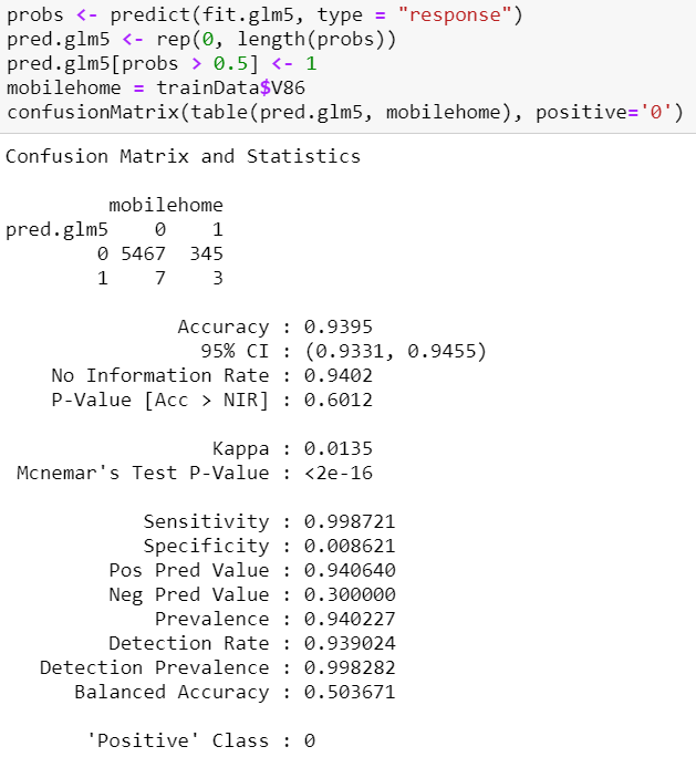
We create a confusion matrix to show how many predictions this model has made correctly and incorrectly in our training dataset.
我们创建一个混淆矩阵,以显示该模型在我们的训练数据集中正确和不正确地做出了多少个预测。
The sensitivity increased slightly from 99.8% to 99.9%. The specificity decreased slightly from 1.44% to 0.8621%.
灵敏度从99.8%略微提高到99.9%。 特异性从1.44%略降至0.8621%。
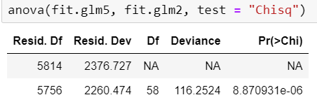
We can run the anova() function to compare this model and the 2nd model and see if they are statistically different.
我们可以运行anova()函数比较此模型和第二个模型,看看它们在统计上是否不同。
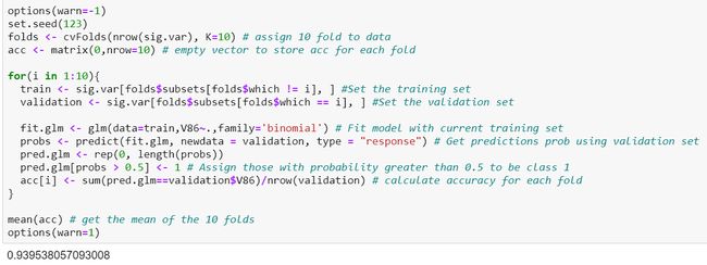
The anova test shows that this model is statistically different compared to the 2nd model since p-value is low (i.e. <0.05). Again, we use 10-Fold Cross Validation Sampling Method to check our accuracy of the model.
方差分析表明,由于p值较低(即<0.05),因此该模型与第二模型相比在统计学上有所不同。 同样,我们使用10倍交叉验证抽样方法来检查模型的准确性。
The cross-validated accuracy is the highest thus far, and is slightly higher than the 2nd model at 0.9385.
交叉验证的准确性是迄今为止最高的,略高于第二个模型的0.9385。
We can consider the variance inflation factors to see if there are any variables that we can consider to remove to simplify our model.
我们可以考虑方差膨胀因子,以查看是否存在可以考虑删除的变量以简化模型。
Variance Inflation Factor is a measure of how much the variance of the estimated regression coefficient is “inflated” by the existence of correlation among the predictor variables in the model.
方差膨胀因子是通过模型中预测变量之间相关性的存在来“估计”估计的回归系数的方差多少的度量。
A VIF of 1 means that there is no correlation among the k-th predictor and the remaining predictor variables, and hence the variance of the k-th coefficient is not inflated at all. The general rule of thumb is that VIFs exceeding 4 warrant further investigation, while VIFs exceeding 10 are signs of serious multicollinearity requiring correction.
VIF为1意味着第k个预测变量与其余的预测变量之间没有相关性,因此第k个系数的方差根本没有被夸大。 一般的经验法则是,超过4的VIF值得进一步研究,而超过10的VIF则表明存在严重的多重共线性,需要纠正。
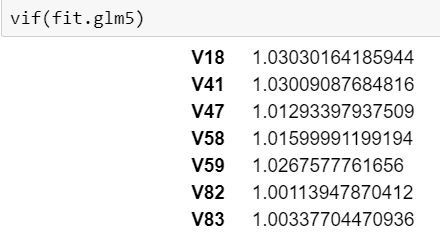
We use the vif function from the car library to determine the VIF.
我们使用car库中的vif函数确定VIF。
As seen, all the 7 variables that were fitted in the 5th model have VIF of around 1 which means there is no correlation among the k-th predictor and the remaining predictor variables. Hence, we will stick to the same model parameters and keep it as the best model for our logistic regression.
如图所示,在第5个模型中拟合的所有7个变量的VIF均约为1,这意味着第k个预测变量与其余预测变量之间没有相关性。 因此,我们将坚持相同的模型参数,并将其保持为逻辑回归的最佳模型。
线性判别分析模型开发1 (Linear Discriminant Analysis model development 1)
The 2nd type of model we can consider is Linear Discriminant Analysis (LDA) which is closely connected to Logistic Regression in which both produce linear decision boundaries that separate a class from another. The only difference is LDA will assume that the observations are drawn from Gaussian Distribution with a common covariance matrix in each class, and if this assumption is true, it will perform better than the Logisitc Regression.
我们可以考虑的第二种类型的模型是线性判别分析(LDA),它与Logistic回归密切相关,其中两者都产生将一个类与另一个类分开的线性决策边界。 唯一的区别是LDA会假设观察是从高斯分布中提取的,并且每个类别中都有一个共同的协方差矩阵,并且如果此假设为真,则其表现将比Logisitc回归更好。
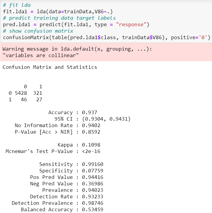
We first fit a LDA model with the full set of variables using lda function from the MASS library and show the confusion matrix to find out the specificity and sensitivity.
我们首先使用MASS库中的lda函数将LDA模型与所有变量集拟合,然后显示混淆矩阵以找出特异性和敏感性。
We see that the sensitivity is 99.2% and specificity 7.8%. Comparing this full LDA model with the full Logistic Regression model, although the sensitivity of the LDA model is lower, it’s specificity is higher than 2.01% in the full Logisitic Regression model. If two or more variables are almost a linear combination to each other, their estimated coefficients will be close to 0 which makes it hard to interpret entirely their effects on the target variable. It is worthy to note that we should avoid variables that are highly correlated to each other in fitting LDA.
我们发现敏感性为99.2%,特异性为7.8%。 将此完整LDA模型与完整Logistic回归模型进行比较,尽管LDA模型的灵敏度较低,但在完整Logisitic回归模型中其特异性高于2.01%。 如果两个或多个变量彼此几乎是线性组合,则它们的估计系数将接近0,这使得很难完全解释它们对目标变量的影响。 值得注意的是,在拟合LDA时,应避免使用彼此高度相关的变量。
Also note that there is a warning message of “variables are collinear” while fitting the LDA model with the full dataset which means some of our predictor variables are correlated to each other which was what was already explored in the EDA section.
还要注意,在将LDA模型与完整数据集拟合时,会出现“变量是共线的”警告消息,这意味着我们的某些预测变量彼此相关,这在EDA部分已经进行了探讨。
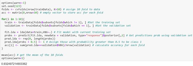
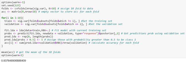
Let’s use 10-Fold Cross Validation Sampling method to get the accuracy of the this model.
让我们使用10倍交叉验证采样方法来获得此模型的准确性。
The accuracy of this model is 93.25%. If we were to compare this model to the models fitted in the logistic regression, this model is currently the best in terms of specificity as it is able to predict correctly 7.76% of the customers who indeed bought mobile home policies, which is the main aim for our prediction task, although the accuracy of the this model is lower than all the models in logistic regression.
该模型的准确性为93.25%。 如果我们将该模型与逻辑回归中的模型进行比较,则该模型目前在特异性方面是最好的,因为它可以正确预测确实购买了移动房屋保单的客户的7.76%,这是主要目标对于我们的预测任务,尽管此模型的准确性低于逻辑回归中的所有模型。
线性判别分析模型开发2 (Linear Discriminant Analysis model development 2)
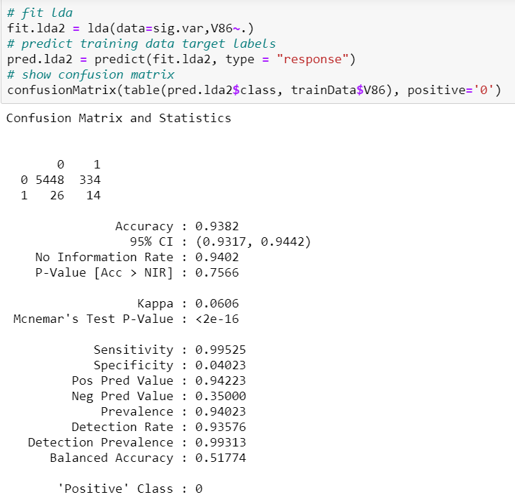
Next, we try to fit the 7 variables that were identified in Logistic Regression model development which performed the best in terms of model complexity and testing specificity.
接下来,我们尝试拟合Logistic回归模型开发中确定的7个变量,它们在模型复杂性和测试特异性方面表现最佳。
Sensitivity is 99.5% and specificity 4.02%. ROC (balanced accuracy) is 0.518. This model performs worse in terms of specificity and better in terms of sensitivity than the full LDA model.
敏感性为99.5%,特异性为4.02%。 ROC(平衡精度)为0.518。 与完整的LDA模型相比,此模型在特异性方面的表现较差,而在灵敏度方面则更好。
Note that we did not receive the warning message of “variables are collinear” in this model as the 7 variables fitted between them has non-significant correlation between them, which was explored in the Variable Inflation Factor (VIF).
请注意,在此模型中我们没有收到“变量是共线的”警告消息,因为它们之间拟合的7个变量之间没有显着的相关性,这在变量通胀因子(VIF)中进行了探讨。
Let’s perform 10 Fold Cross Validation to get the mean accuracy of this model.
让我们执行10次折叠交叉验证以获取该模型的平均准确性。
Accuracy of this model is 0.9376 which is higher than the previous model at 0.9325, but still lower than all the models in logistic regression.
该模型的精度为0.9376,高于先前模型的0.9325,但仍低于逻辑回归中的所有模型。
二次判别分析模型开发1 (Quadratic Discriminant Analysis model development 1)
The 3rd type of model we can consider is Quadratic Discriminant Analysis (QDA). In Linear Discriminant Analysis, we assume that the observations are drawn from Gaussian Distribution with a common covariance matrix in each class. However in QDA, this assumption does not hold as each class is allowed to have different covariance matrix.
我们可以考虑的第三种模型是二次判别分析(QDA)。 在线性判别分析中,我们假设观测值是从高斯分布中得出的,每个类别中都有一个共同的协方差矩阵。 但是在QDA中,此假设不成立,因为允许每个类别具有不同的协方差矩阵。
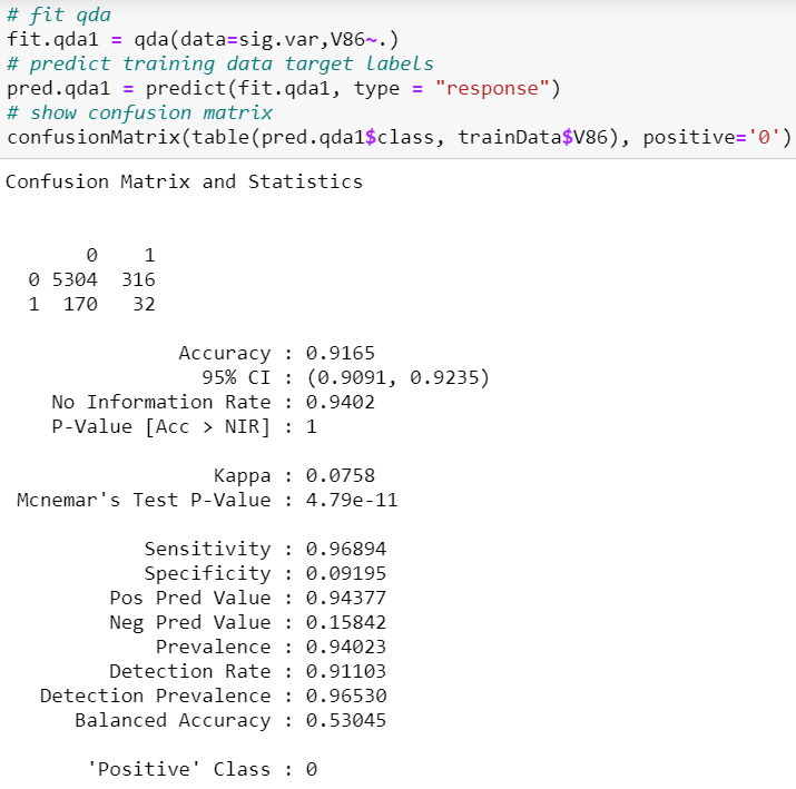
In both of our Logistic Regression and Linear Discriminant Analysis model development, we found out that the best model respectively is the one using the 7 variables that were deemed significant from Lasso regression, Forward Stepwise Selection and Backward Stepwise Selection. Hence, we first train our QDA model using this set of 7 variables.
在我们的Logistic回归和线性判别分析模型开发中,我们发现最佳模型分别是使用从Lasso回归,正向逐步选择和向后逐步选择中被认为是重要的7个变量的模型。 因此,我们首先使用这7个变量集训练我们的QDA模型。
Sensitivity is 96.89% which is the lowest thus far out of all the models trained. Specificity is 9.20% which is the highest out of all models thus far.
灵敏度为96.89%,是迄今为止所有训练模型中最低的。 特异性为9.20%,是迄今为止所有模型中最高的。
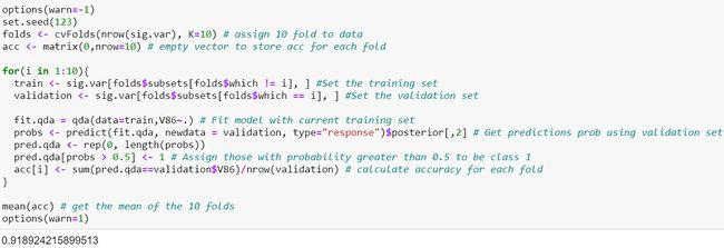
Let’s get the mean accuracy of this model from 10-Fold Cross Validation.
让我们从十折交叉验证中获得该模型的平均准确性。
Accuracy of model is 0.9189 which is the lowest thus far out of all the models that have been trained.
模型的准确性是0.9189,是迄今为止所有已训练模型中最低的。
Since the accuracy of QDA appears to be lower than both Logistic Regression and Linear Discriminant Analysis model, we will not train any more models with QDA.
由于QDA的准确性似乎低于Logistic回归和线性判别分析模型,因此我们将不再使用QDA训练模型。
选择模型 (Chosen Model)
Comparing these 3 models, the best model we will choose for our prediction task will the 2nd model of Linear Discriminant Analysis containing the set of predictor variables (V18, V41, V47, V58, V59, V82, V83) that were identified as significant from the first 4 Logistic Regression Models. Firstly, even though the CV accuracy is lower compared to other models in Logistic Regression, it’s specificity is the highest. Since the task is to find the subset of customers who are likely to purchase caravan policies so that the rest who don’t will receive a mailing, our aim will be to maximise the identification of this group of customers who are likely to purchase mobile home policies so that the insurance company can save cost on the mailing who a smaller group of customers who are identified as not likely to purchase the mobile home policies, which means we will be looking more on specificity of the model. Although the specificity of the QDA model is the highest, the CV accuracy for the QDA model is very low. As a result, we chose the 2nd model in LDA as the best model for our prediction task as we want something in between for accuracy and specificity.
比较这三个模型,我们将为预测任务选择的最佳模型是线性判别分析的第二个模型,该模型包含一组预测变量(V18,V41,V47,V58,V59,V82,V83),这些变量在前4个Logistic回归模型。 首先,尽管与Logistic回归中的其他模型相比,CV准确性较低,但它的特异性最高。 由于任务是找到可能购买房车保单的客户子集,以便其余未收到邮寄保单的客户,我们的目标是最大程度地识别这组可能购买移动房屋的客户这样,保险公司就可以节省邮寄费用,而这笔费用被确定为不太可能购买移动房屋保单的较小客户群,这意味着我们将更多地关注模型的特异性。 尽管QDA模型的特异性最高,但QDA模型的CV准确性却很低。 结果,我们选择了LDA中的第二个模型作为预测任务的最佳模型,因为我们希望在准确性和特异性之间取得一些优势。
Prediction using testing dataset
使用测试数据集进行预测
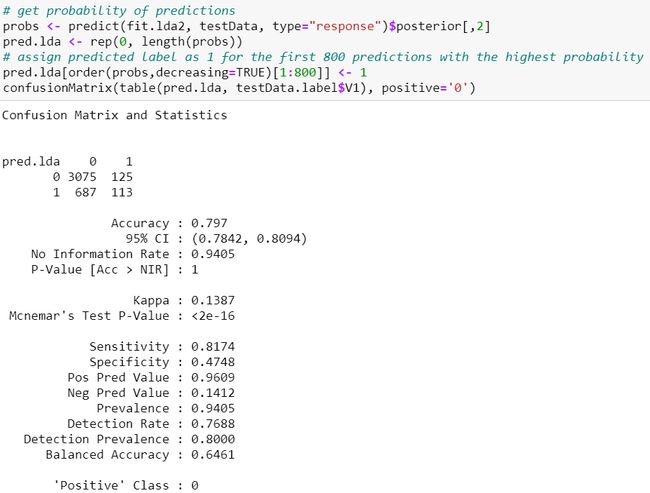
We are also provided with the testing dataset and we can use it to see how well will the LDA model we have identified as best perform. We are supposed to find a set of 800 customers in this testing dataset that are most likely to purchase mobile home policies based on the probabilities predicted by our model. After identifying this set of 800 customers, we then use the true testing data target values and see how many of them are identified correctly and incorrectly. Note that in real life problems, all we may have is a set of data which we have to use method like 70:30 split for us to get training and testing data in order to test our ML algorithms.
我们还提供了测试数据集,我们可以使用它来查看我们确定为最佳性能的LDA模型的性能。 我们应该在此测试数据集中找到800个客户,这些客户最有可能根据模型预测的概率购买移动房屋保单。 在确定这800个客户组之后,我们将使用真实的测试数据目标值,并查看正确和不正确地确定了其中的多少。 请注意,在现实生活中的问题中,我们可能只有一组数据,我们必须使用70:30 split这样的方法来获取训练和测试数据,以便测试ML算法。
The accuracy of our model using testing dataset is 79.7% in which it’s sensitivity was 81.74% and specificity 47.48%. Out of a total of 238 actual mobile home policy customers, our model correctly identified 113 of them.
我们使用测试数据集的模型的准确性为79.7%,其中灵敏度为81.74%,特异性为47.48%。 在总共238个实际的移动房屋保单客户中,我们的模型正确地确定了113个客户。
概要 (Summary)
The winner of this challenge came up with an algorithm that was able to identify 121 customers correctly, and ours which successfully identified 113, wasn’t that bad. The standard benchmark tests result in 94 using K-nearest neighbours, 102 using naive bayes and 105 using neural networks, which were all more complicated than our LDA model. Hope you guys enjoy this ML model building walkthrough and have a better sense now on how to approach a problem using exploratory data analysis, feature selection and machine learning!
这项挑战的胜者提出了一种算法,该算法能够正确识别121位客户,而我们的算法成功识别了113位客户,还算不错。 标准基准测试的结果是使用K近邻的有94个,使用朴素贝叶斯的有102个,使用神经网络的105个,这比我们的LDA模型要复杂得多。 希望大家喜欢这个ML模型构建演练,并且现在对如何使用探索性数据分析,特征选择和机器学习解决问题有了更好的认识!
翻译自: https://medium.com/swlh/machine-learning-to-kaggle-caravan-insurance-challenge-on-r-f52790bc7669
