YOLO V1 算法详解与PyTorch复现
[本文中的代码有部分是描述性代码,如需完整项目请参考github地址-见本文底部,另外,该复现版本还在测试优化中~]
1. YOLO v1概述
Two-stage目标检测算法将目标检测与识别的过程分为候选区域提取与目标识别两个步骤来做,由于在做具体分类识别和位置回归前多了一步候选区域提取,因此Two-stage目标检测算法的识别率和候选框精确度是比较高的,但对性能的消耗是非常巨大的。而YOLO v1作为YOLO系列算法的开山之作,创造性地提出不再预先进行候选区域(Proposal Region)的提取,而是直接将输入图片以网格的方式进行划分,由每个网格负责预测中心点落在它内部的物体。不过也正是因为缺少了Proposal Region的提取,所以相对来说回归精度要低一些。Yolo v1是端到端的,直接做预测,而不是通过候选区域提取,将目标检测问题转换为一个分类问题。
| One-stage | Two-stage |
| 优点 | 优点 |
| 推理速度快、训练快 | 精度高 |
| 背景误检率低 | 目标定位精度高 、检出率高 |
| 缺点 | 缺点 |
| 目标定位精度低 、检出率低 | 推理速度慢、训练慢 |
| 小物体检测效果差 | 背景误检率高 |
2.YOLO v1网络结构
作者实现的YOLO v1版本中,输入图像的尺寸固定为448*448,在经过了24个卷积层和2个全连接层后,最后输出7*7*1024的特征图(feature map),对应了作者将原图划分为S*S个格子的思想,feature map上的每一个张量都包含了后续预测任务时所需要的高层抽象语意信息。

如图,YOLO v1将一张图片划分为S*S个格子,作者称之为栅格(grid cell)。对于一张大小为448*448的图像,经卷积层提取特征后,输出大小为7*7*1024的特征图(feature map),feature map上的每一个1*1*1024的张量就对应着原图中的一个grid cell所提取出的特征,不同的通道对应着不同的抽象语意信息。每个grid cell预测两个物体边界框(Bounding Box)以及grid cell预测的物体类别,最后通过一个NSM算法去除冗余的Bounding Box,生成检测结果。

如图, YOLO v1的网络架构为24个卷积层、4个最大池化层、2个全连接层组成,卷积和池化层部分用于特征的提取,全连接层用于预测。全连接层输出7*7*30,7*7代表原图被划分成的7*7的grid cell。
Yolo_v1_model.py:
import torch.nn as nn

class Convention(nn.Module):
    def __init__(self,in_channels,out_channels,conv_size,conv_stride,padding):
        super(Convention,self).__init__()
        self.Conv = nn.Sequential(
            nn.Conv2d(in_channels, out_channels, conv_size, conv_stride, padding),
            nn.BatchNorm2d(out_channels),
            nn.LeakyReLU()
        )

    def forward(self, x):
        return self.Conv(x)

class YOLO_V1(nn.Module):

    def __init__(self,B=2,Classes_Num=20):
        super(YOLO_V1,self).__init__()
        self.B = B
        self.Classes_Num = Classes_Num

        self.Conv_448 = nn.Sequential(
            Convention(3, 64, 7, 2, 3),
            nn.MaxPool2d(2,2),
        )

        self.Conv_112 = nn.Sequential(
            Convention(64, 192, 3, 1, 1),
            nn.MaxPool2d(2, 2),
        )

        self.Conv_56 = nn.Sequential(
            Convention(192, 128, 1, 1, 0),
            Convention(128, 256, 3, 1, 1),
            Convention(256, 256, 1, 1, 0),
            Convention(256, 512, 3, 1, 1),
            nn.MaxPool2d(2, 2),
        )

        self.Conv_28 = nn.Sequential(
            Convention(512, 256, 1, 1, 0),
            Convention(256, 512, 3, 1, 1),
            Convention(512, 256, 1, 1, 0),
            Convention(256, 512, 3, 1, 1),
            Convention(512, 256, 1, 1, 0),
            Convention(256, 512, 3, 1, 1),
            Convention(512, 256, 1, 1, 0),
            Convention(256, 512, 3, 1, 1),
            Convention(512,512,1,1,0),
            Convention(512,1024,3,1,1),
            nn.MaxPool2d(2, 2),
        )

        self.Conv_14 = nn.Sequential(
            Convention(1024,512,1,1,0),
            Convention(512,1024,3,1,1),
            Convention(1024, 512, 1, 1, 0),
            Convention(512, 1024, 3, 1, 1),
            Convention(1024, 1024, 3, 1, 1),
            Convention(1024, 1024, 3, 2, 1),
        )

        self.Conv_7 = nn.Sequential(
            Convention(1024,1024,3,1,1),
            Convention(1024, 1024, 3, 1, 1),
        )

        self.Fc = nn.Sequential(
            nn.Dropout(0.5),
            nn.Linear(7*7*1024,4096),
            nn.ReLU(),
            nn.Dropout(0.5),
            nn.Linear(4096,7 * 7 * (B*5 + Classes_Num)),
            nn.Sigmoid()
        )

    def forward(self, x):
        x = self.Conv_448(x)
        x = self.Conv_112(x)
        x = self.Conv_56(x)
        x = self.Conv_28(x)
        x = self.Conv_14(x)
        x = self.Conv_7(x)
        # batch_size * channel * height * weight -> batch_size * height * weight * channel
        x = x.permute(0,2,3,1).contiguous()
        x = x.view(-1,7*7*1024)
        x = self.Fc(x)
        x = x.view((-1,7,7,(self.B*5 + self.Classes_Num)))
        return x
3.YOLO v1输出结果

如图,由于作者使用了VOC数据集(20个类别)来测试并测试YOLO v1,所以预测输出的张量中,前面两个5维分别表示两个Bounding Box的物体置信度以及两个box各自的中心坐标及宽高,后面的20维对应了20种类别各自的概率。
IOU:(区域交并比)

在目标检测领域,IoU是一个重要指标,通过两个box的交集和并集的面积值比值来衡量两个boxes的接近程度(重叠程度)。
矩形交集计算:https://blog.csdn.net/qq_39304630/article/details/112759739
def iou(self, box1, box2):  # 计算两个box的IoU值
    # box: lx-左上x ly-左上y rx-右下x ry-右下y 图像向右为y 向下为x
    # 1. 获取交集的矩形左上和右下坐标
    interLX = max(box1[0],box2[0])
    interLY = max(box1[1],box2[1])
    interRX = min(box1[2],box2[2])
    interRY = min(box1[3],box2[3])

    # 2. 计算两个矩形各自的面积
    Area1 = (box1[2] - box1[0]) * (box1[3] - box1[1])
    Area2 = (box2[2] - box2[0]) * (box2[3] - box2[1])

    # 3. 不存在交集
    if interRX < interLX or interRY < interLY:
        return 0

    # 4. 计算IOU
    interSection = (interRX - interLX) * (interRY - interLY)
return interSection / (Area1 + Area2 - interSection)置信度:作者采用了同时考虑有无物体以及定位准确度的方式
![]()
![]() 表示有物体的中心落在当前的grid cell内部的概率,即当前grid cell负责的区域有物体的概率。
表示有物体的中心落在当前的grid cell内部的概率,即当前grid cell负责的区域有物体的概率。![]() 表示当前用于预测的Bounding Box与真实要预测的物体的Truth Box的IOU值,这体现了预测的Bounding Box的准确度。
表示当前用于预测的Bounding Box与真实要预测的物体的Truth Box的IOU值,这体现了预测的Bounding Box的准确度。
预测输出的![]() 表示Bounding Box覆盖的区域含有物体的可能性,而我们在制作Ground Truth时,如果该grid cell中有物体的中心,则该Ground Truth的
表示Bounding Box覆盖的区域含有物体的可能性,而我们在制作Ground Truth时,如果该grid cell中有物体的中心,则该Ground Truth的![]() =1,否则
=1,否则![]() =0。
=0。
定位:如果我们直接预测Bounding Box的位置、长宽,这会导致模型的泛化能力有所降低,这是因为:
1. 直接预测图像中心点的位置和尺度,会导致预测值的变化幅度占据了[0,447],尺度变化太过剧烈,并不利于网络的收敛,训练过程中波动会很大
2. 如果网络训练和测试的图片中物体的尺度差异过大,会导致模型在测试数据上的识别能力完全不够
因此作者使用了相对偏移量的方式,由于每一个grid cell 负责预测目标中心落在其内部的物体,因此物体中心的坐标一定在grid cell内,所以将中心点与grid cell左上角的坐标差与grid cell本身的长宽做除法得到相对的比例值。同样,物体的长宽预测,由于物体一定落在整个图像内部,于是可以与图像的长宽做除法得到相对的比例值,如下图:

预测输出的结果我们使用sigmod函数将输出压缩在(0,1),在制作Ground Truth时,我们根据上述约定直接计算即可。
Yolo_V1_DataSet.py
from torch.utils.data import Dataset
import os
import cv2
import xml.etree.ElementTree as ET
import torch
import torchvision.transforms as transforms

class YoloV1DataSet(Dataset):

    def __init__(self, imgs_dir="./VOC2007/Train/JPEGImages", annotations_dir="./VOC2007/Train/Annotations", img_size=448, S=7, B=2, ClassesFile="./VOC2007/Train/class.data"): # 图片路径、注解文件路径、图片尺寸、每个grid cell预测的box数量、类别文件
        img_names = os.listdir(imgs_dir)
        img_names.sort()
        self.transfrom = transforms.Compose([
            transforms.ToTensor(), # height * width * channel -> channel * height * width
            transforms.Normalize(mean=(0.5,0.5,0.5),std=(0.5,0.5,0.5))
        ])
        self.img_path = []
        for img_name in img_names:
            self.img_path.append(os.path.join(imgs_dir,img_name))
        annotation_names = os.listdir(annotations_dir)
        annotation_names.sort() #图片和文件排序后可以按照相同索引对应
        self.annotation_path = []
        for annotation_name in annotation_names:
            self.annotation_path.append(os.path.join(annotations_dir,annotation_name))
        self.img_size = img_size
        self.S = S
        self.B = B
        self.grid_cell_size = self.img_size / self.S
        self.ClassNameToInt = {}
        classIndex = 0
        with open(ClassesFile, 'r') as f:
            for line in f:
                line = line.replace('\n','')
                self.ClassNameToInt[line] = classIndex #根据类别名制作索引
                classIndex = classIndex + 1
        print(self.ClassNameToInt)
        self.Classes = classIndex # 一共的类别个数
        self.getGroundTruth()

    # PyTorch 无法将长短不一的list合并为一个Tensor
    def getGroundTruth(self):
        self.ground_truth = [[[list() for i in range(self.S)] for j in range(self.S)] for k in
                             range(len(self.img_path))]  # 根据标注文件生成ground_truth
        ground_truth_index = 0
        for annotation_file in self.annotation_path:
            ground_truth = [[list() for i in range(self.S)] for j in range(self.S)]
            # 解析xml文件--标注文件
            tree = ET.parse(annotation_file)
            annotation_xml = tree.getroot()
            # 计算 目标尺寸 -> 原图尺寸 self.img_size * self.img_size , x的变化比例
            width = (int)(annotation_xml.find("size").find("width").text)
            scaleX = self.img_size / width
            # 计算 目标尺寸 -> 原图尺寸 self.img_size * self.img_size , y的变化比例
            height = (int)(annotation_xml.find("size").find("height").text)
            scaleY = self.img_size / height
            # 因为两次除法的误差可能比较大 这边采用除一次乘一次的方式
            # 一个注解文件可能有多个object标签,一个object标签内部包含一个bnd标签
            objects_xml = annotation_xml.findall("object")
            for object_xml in objects_xml:
                # 获取目标的名字
                class_name = object_xml.find("name").text
                if class_name not in self.ClassNameToInt: # 不属于我们规定的类
                    continue
                bnd_xml = object_xml.find("bndbox")
                # 目标尺度放缩
                xmin = (int)((int)(bnd_xml.find("xmin").text) * scaleX)
                ymin = (int)((int)(bnd_xml.find("ymin").text) * scaleY)
                xmax = (int)((int)(bnd_xml.find("xmax").text) * scaleX)
                ymax = (int)((int)(bnd_xml.find("ymax").text) * scaleY)
                # 目标中心点
                centerX = (xmin + xmax) / 2
                centerY = (ymin + ymax) / 2
                # 当前物体的中心点落于 第indexI行 第indexJ列的 grid cell内
                indexI = (int)(centerY / self.grid_cell_size)
                indexJ = (int)(centerX / self.grid_cell_size)
                # 真实物体的list
                ClassIndex = self.ClassNameToInt[class_name]
                ClassList = [0 for i in range(self.Classes)]
                ClassList[ClassIndex] = 1
                ground_box = list([centerX / self.grid_cell_size - indexJ,centerY / self.grid_cell_size - indexI,(xmax-xmin)/self.img_size,(ymax-ymin)/self.img_size,1,xmin,ymin,xmax,ymax,(xmax-xmin)*(ymax-ymin)])
                #增加上类别
                ground_box.extend(ClassList)
                ground_truth[indexI][indexJ].append(ground_box)

            #同一个grid cell内的多个groudn_truth,选取面积最大的两个
            for i in range(self.S):
                for j in range(self.S):
                    if len(ground_truth[i][j]) == 0:
                        self.ground_truth[ground_truth_index][i][j].append([0 for i in range(10 + self.Classes)])
                    else:
                        ground_truth[i][j].sort(key = lambda box: box[9], reverse=True)
                        self.ground_truth[ground_truth_index][i][j].append(ground_truth[i][j][0])

            ground_truth_index = ground_truth_index + 1
        self.ground_truth = torch.Tensor(self.ground_truth).float()

    def __getitem__(self, item):
        # height * width * channel
        img_data = cv2.imread(self.img_path[item])
        img_data = cv2.resize(img_data, (448, 448), interpolation=cv2.INTER_AREA)
        img_data = self.transfrom(img_data)
        return img_data,self.ground_truth[item]


    def __len__(self):
        return len(self.img_path)
[注]:在YOLO v1中,每一个grid cell虽然预测两个bounding box,但是最终只有一个是有效的,最多检测7*7*1=49个物体,因此在本人的实现中,对于多个物体的重心落于同一个grid cell的情况,采用的方式是选择具有最大面积的物体。
4. YOLO v1 损失函数
损失函数是深度学习网络模型非常重要的“指挥棒”,负责引导整体网络的任务和学习方向,通过对预测样本和真实样本的误差进行反向传播来指导网络进行参数的调整学习。
我们将含有物体的Bounding Box当作正样本,将不含有物体的Bounding Box当作负样本。在实际的实现上,通过Bounding Box与真实的物体边界框(Ground Truth)的IoU值来判定正负样本,将与Ground Truth拥有最大IoU值的box当作正样本,其余的box作为负样本。
整个YOLO v1算法的损失函数就包含分别关于正样本(负责预测物体的Bounding Box)和负样本(负责预测物体的Bounding Box)两部分,正样本置信度为1,负样本置信度为0,正样本的损失包含置信度损失、边框回归损失和类别损失,而负样本损失只有置信度损失。
[注]:这边解释一下,因为我们预先设置好了S*S*B个Bounding Box,但是有可能存在一些Bounding Box是完全没有预测到目标的,那些预测到目标的Bounding Box就是正样本,没有预测到目标的就是负样本。在作者创作YOLO v1的那个年代,用于目标检测的数据还没有特别密集的目标的情况,因此存在较多的负样本。
YOLO v1的损失由5个部分组成,均使用均方差损失:
(1) 第一部分为正样本中心点坐标的损失,引入![]()
![]() 参数调节定位损失的权重。默认设置为5,提高了定位损失的权重,避免在训练初期,由于负样本过多导致正样本的损失在反向传播时的作用微弱进而导致模型不稳定、网络训练发散的问题。
参数调节定位损失的权重。默认设置为5,提高了定位损失的权重,避免在训练初期,由于负样本过多导致正样本的损失在反向传播时的作用微弱进而导致模型不稳定、网络训练发散的问题。
![\lambda coord\sum_{i=0}^{S*S}\sum_{j=0}^{B}1_{ij}^{obj}[(x_{i}-\hat{x}_{i})^{2}+(y_{i}-\hat{y}_{i})^{2}]](http://img.e-com-net.com/image/info8/25978464e105483588531f06373542ca.gif)
![]() :超参数,用于调节定位损失在整体损失中的权重
:超参数,用于调节定位损失在整体损失中的权重
![]() :S*S个格子里都有Bounding Box
:S*S个格子里都有Bounding Box
![]() :每个格子里有B个Bounding Box
:每个格子里有B个Bounding Box
![]() :第i个网格中的第j个Bounding Box负责预测该网格对应的物体时为1,否则为0
:第i个网格中的第j个Bounding Box负责预测该网格对应的物体时为1,否则为0
![]() :物体中心点与Bounding Box预测的中心点的差距
:物体中心点与Bounding Box预测的中心点的差距
(2) 第二部分为正样本的宽高损失,YOLO v1通过对宽高进行根号处理,在一定程度上降低了网络对尺度变化的敏感程度,同时也能提高小物体宽高损失在整体目标宽高差距损失上的权重。毕竟,对于大型的Bounding Box来说,小的偏差影响并不大,而对于小型的Bounding Box来说,小型的偏差就显得尤为重要。
![\lambda coord\sum_{i=0}^{S*S}\sum_{j=0}^{B}1_{ij}^{obj}[(\sqrt{w_{i}}-\sqrt{\hat{w}_{i}})^{2}+(\sqrt{h_{i}}-\sqrt{\hat{h}_{i}})^{2}]](http://img.e-com-net.com/image/info8/8e610be298d240cbb6a46f4ec1b253c6.gif)
![]() :物体的长宽与Bounding Box预测的长宽之间的差距,根号处理是因为小尺度的目标对于尺度变化很敏感。例如,目标尺度为10,预测出来为20,差值为100%;目标尺度为100,预测出来为110,插值为10%。
:物体的长宽与Bounding Box预测的长宽之间的差距,根号处理是因为小尺度的目标对于尺度变化很敏感。例如,目标尺度为10,预测出来为20,差值为100%;目标尺度为100,预测出来为110,插值为10%。
(3) 第三部分分别为正样本的置信度损失。

![]() :含有物体的Bounding Box的置信度与对应Ground Truth的置信度方差
:含有物体的Bounding Box的置信度与对应Ground Truth的置信度方差
(4) 第四部分为负样本的置信度损失,引入![]() 调节负样本置信度损失的权重,默认值为0.5。
调节负样本置信度损失的权重,默认值为0.5。
![]() :由于负样本常常比较多,为了保证网络更多的还是学习如果正确定位正样本,因此需要将负样本的损失权重降低
:由于负样本常常比较多,为了保证网络更多的还是学习如果正确定位正样本,因此需要将负样本的损失权重降低
![]() :不含有物体的Bounding Box的置信度与对应Ground Truth的置信度方差
:不含有物体的Bounding Box的置信度与对应Ground Truth的置信度方差
(5) 第五部分是正样本的类别损失。
![]()
![]() :是否有物体的中心落在该grid cell中
:是否有物体的中心落在该grid cell中
![]() :对于每一个类别,都计算平方误差
:对于每一个类别,都计算平方误差
Yolo_v1_lossFunction.py
import torch.nn as nn
import math
import torch

class Yolov1_Loss(nn.Module):

    def __init__(self, S=7, B=2, Classes=20, l_coord=5, l_noobj=0.5):
        # 有物体的box损失权重设为l_coord,没有物体的box损失权重设置为l_noobj
        super(Yolov1_Loss, self).__init__()
        self.S = S
        self.B = B
        self.Classes = Classes
        self.l_coord = l_coord
        self.l_noobj = l_noobj

    def iou(self, bounding_box, ground_box, gridX, gridY, img_size=448, grid_size=64):  # 计算两个box的IoU值
        # predict_box: [centerX, centerY, width, height]
        # ground_box : [centerX / self.grid_cell_size - indexJ,centerY / self.grid_cell_size - indexI,(xmax-xmin)/self.img_size,(ymax-ymin)/self.img_size,1,xmin,ymin,xmax,ymax,(xmax-xmin)*(ymax-ymin)
        # 1.  预处理 predict_box  变为  左上X,Y  右下X,Y  两个边界点的坐标 避免浮点误差 先还原成整数
        # 不要共用引用
        predict_box = list([0,0,0,0])
        predict_box[0] = (int)(gridX + bounding_box[0] * grid_size)
        predict_box[1] = (int)(gridY + bounding_box[1] * grid_size)
        predict_box[2] = (int)(bounding_box[2] * img_size)
        predict_box[3] = (int)(bounding_box[3] * img_size)

        # [xmin,ymin,xmax,ymax]
        predict_coord = list([max(0, predict_box[0] - predict_box[2] / 2), max(0, predict_box[1] - predict_box[3] / 2),min(img_size - 1, predict_box[0] + predict_box[2] / 2), min(img_size - 1, predict_box[1] + predict_box[3] / 2)])
        predict_Area = (predict_coord[2] - predict_coord[0]) * (predict_coord[3] - predict_coord[1])

        ground_coord = list([ground_box[5],ground_box[6],ground_box[7],ground_box[8]])
        ground_Area = (ground_coord[2] - ground_coord[0]) * (ground_coord[3] - ground_coord[1])

        # 存储格式 xmin ymin xmax ymax

        # 2.计算交集的面积 左边的大者 右边的小者 上边的大者 下边的小者
        CrossLX = max(predict_coord[0], ground_coord[0])
        CrossRX = min(predict_coord[2], ground_coord[2])
        CrossUY = max(predict_coord[1], ground_coord[1])
        CrossDY = min(predict_coord[3], ground_coord[3])

        if CrossRX < CrossLX or CrossDY < CrossUY: # 没有交集
            return 0

        interSection = (CrossRX - CrossLX + 1) * (CrossDY - CrossUY + 1)
        return interSection / (predict_Area + ground_Area - interSection)

    def forward(self, bounding_boxes, ground_truth, batch_size=32,grid_size=64, img_size=448):  # 输入是 S * S * ( 2 * B + Classes)
        # 定义三个计算损失的变量 正样本定位损失 样本置信度损失 样本类别损失
        loss = 0
        loss_coord = 0
        loss_confidence = 0
        loss_classes = 0
        iou_sum = 0
        object_num = 0
        mseLoss = nn.MSELoss()
        for batch in range(len(bounding_boxes)):
            for i in range(self.S):  # 先行 - Y
                for j in range(self.S):  # 后列 - X
                    # 取bounding box中置信度更大的框
                    if bounding_boxes[batch][i][j][4] < bounding_boxes[batch][i][j][9]:
                        predict_box = bounding_boxes[batch][i][j][5:]
                        # 另一个框是负样本
                        loss = loss + self.l_noobj * torch.pow(bounding_boxes[batch][i][j][4], 2)
                        loss_confidence += self.l_noobj * math.pow(bounding_boxes[batch][i][j][4].item(), 2)
                    else:
                        predict_box = bounding_boxes[batch][i][j][0:5]
                        predict_box = torch.cat((predict_box, bounding_boxes[batch][i][j][10:]), dim=0)
                        # 另一个框是负样本
                        loss = loss + self.l_noobj * torch.pow(bounding_boxes[batch][i][j][9], 2)
                        loss_confidence += self.l_noobj * math.pow(bounding_boxes[batch][i][j][9].item(), 2)
                    # 为拥有最大置信度的bounding_box找到最大iou的groundtruth_box
                    if ground_truth[batch][i][j][0][9] == 0:  # 面积为0的grount_truth 为了形状相同强行拼接的无用的0-box negative-sample
                        loss = loss + self.l_noobj * torch.pow(predict_box[4], 2)
                        loss_confidence += self.l_noobj * math.pow(predict_box[4].item(), 2)
                    else:
                        object_num = object_num + 1
                        iou = self.iou(predict_box, ground_truth[batch][i][j][0], j * 64, i * 64)
                        iou_sum = iou_sum + iou
                        ground_box = ground_truth[batch][i][j][0]
                        loss = loss + self.l_coord * (torch.pow((ground_box[0] - predict_box[0]), 2) + torch.pow((ground_box[1] - predict_box[1]), 2) + torch.pow(torch.sqrt(ground_box[2] + 1e-8) - torch.sqrt(predict_box[2] + 1e-8), 2) + torch.pow(torch.sqrt(ground_box[3] + 1e-8) - torch.sqrt(predict_box[3] + 1e-8), 2))
                        loss_coord += self.l_coord * (math.pow((ground_box[0] - predict_box[0]), 2) + math.pow((ground_box[1] - predict_box[1]), 2) + math.pow(math.sqrt(ground_box[2] + 1e-8) - math.sqrt(predict_box[2] + 1e-8), 2) + math.pow(math.sqrt(ground_box[3] + 1e-8) - math.sqrt(predict_box[3] + 1e-8), 2))
                        loss = loss + torch.pow(ground_box[4] - predict_box[4], 2)
                        loss_confidence += math.pow(ground_box[4] - predict_box[4], 2)
                        ground_class = ground_box[10:]
                        predict_class = bounding_boxes[batch][i][j][self.B * 5:]
                        loss = loss + mseLoss(ground_class,predict_class) * self.Classes
                        loss_classes += mseLoss(ground_class,predict_class).item() * self.Classes
        print("坐标误差:{} 置信度误差:{} 类别损失:{} iou_sum:{} object_num:{} iou:{}".format(loss_coord, loss_confidence, loss_classes, iou_sum, object_num, "nan" if object_num == 0 else (iou_sum / object_num)))
        return loss, loss_coord, loss_confidence, loss_classes, iou_sum, object_num
[注]:的确可能存在一个grid cell中含有多个物体的中心点的情况,本人的处理策略为选取具有最大面积的那个ground_truth,降低网络训练的难度,因为YOLO v1天生就存在着小物体识别能力不足的缺陷。
5. YOLO v1预测结果处理--NMS算法
通常来说,目标检测算法的最终输出结果是很多的Bounding Box用于预测目标,常用做法是将所有的Box通过非极大值抑制(NMS)算法去除冗余,保留效果最好的。
| 算法 NMS算法 |
| 输入:Bounding Box的集合p、IoU阈值、置信度阈值。 输出:去除冗余的Bounding box集合q。 1.去除集合p中置信度低于置信度阈值的Bounding Box。 2.在集合p中选取拥有最大置信度的Box,移出集合p并加入集合q,并将p中剩余的Bounding Box与该box计算IOU值,去除那些与该Box的IOU值超过阈值的Bounding Box。 3.重复步骤2,直到集合p为空 4.输出集合q,为所求的结果集合。 |
NMS.py
import numpy as np

# 这边要求的bounding_boxes为处理后的实际的样子
def NMS(bounding_boxes,confidence_threshold,iou_threshold):
    # boxRow : x y dx dy c
    # 1. 初步筛选,先把grid cell预测的两个bounding box取出置信度较高的那个
    boxes = []
    for boxRow in bounding_boxes:
        # grid cell预测出的两个box,含有物体的置信度没有达到阈值
        if boxRow[4] < confidence_threshold or boxRow[9] < confidence_threshold:
            continue
        # 获取物体的预测概率
        classes = boxRow[10:-1]
        class_probality_index = np.argmax(classes,axis=1)
        class_probality = classes[class_probality_index]
        # 选择拥有更大置信度的box
        if boxRow[4] > boxRow[9]:
            box = boxRow[0:4]
        else:
            box = boxRow[5:9]
        # box : x y dx dy class_probality_index class_probality
        box.append(class_probality_index)
        box.append(class_probality)
        boxes.append(box)

    # 2. 循环直到待筛选的box集合为空
    predicted_boxes = []
    while len(boxes) != 0:
        # 对box集合按照置信度从大到小排序
        boxes = sorted(boxes, key=(lambda x : [x[4]]), reverse=True)
        # 确定含有最大值信度的box会被选中
        choiced_box = boxes[0]
        predicted_boxes.append(choiced_box)
        for index in len(boxes):
            # 如果冲突的box的iou值已经大于阈值 需要丢弃
            if iou(boxes[index],choiced_box) > iou_threshold:
                boxes.pop(index)

    return predicted_boxes
6. YOLO v1分析
1.YOLO v1网络优势
①在3*3的卷积后接上一个通道数低的1*1的卷积,用于进行特征的通道压缩,降低计算量;同时多一层的卷积也提升了模型的非线性表达能力。
②在训练中使用Dropout和数据增强的方式来防止网络过拟合。
③并没有引入Anchor机制,而是直接在每个区域进行框的大小与位置信息的预测,利用区域本身携带的位置信息和被检测物体尺度处于网络可以回归范围之内的特性将目标检测问题转化为一个回归问题。
④YOLO v1将物体类别与物体置信度分开预测,简化了问题,实验证明YOLO v1背景误检率要低于Fast R-CNN,YOLO v1的误差主要来源是定位误差,如图4-7所示:

2.YOLO v1缺陷分析
①每一个区域只预测两个框,并且共用同一个类别向量,这导致YOLO v1只能检测有限个物体,并且对于小物体和距离相近的物体的检测效果并不好,而实际的情况下,预测的7*7*2=98个bounding box中,最多只有49个是有效的,也就是说YOLO v1对于一张图片最多预测49个物体。
②由于没有引入Anchor机制,而是直接从数据中学习并进行预测,故很难泛化到新的、不常见的宽高比例的目标的检测中,所以模型对于新的或者并不常见宽高比例的物体检测效果并不好。另外,由于下采样率比较大,对于边框的回归精度也不高。
③在v1的损失函数设计中,大物体和小物体的定位损失权重一样,这将会导致同等比例的定位误差,大物体的损失会比小物体大,小物体的损失在总损失中占比较小,然而实际上,小边界框的小误差对IoU的影响比大边界框要大得多,会导致定位的不准确,但是作者也是知道的,只不过为了保持YOLO v1简单的特性,作者的处理方式是使用对尺度开方,依此提高小物体尺度损失的相对权重。
3.YOLO v1与其他网络的性能对比:
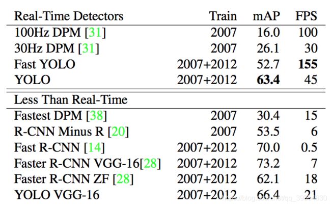
相较于DPM等传统方法而言,YOLO有更高的精度;相较于以Fast R-CNN为代表的一系列的Two-stage算法,YOLO的精度稍有逊色,但是FPS达到了完全碾压的地步,兼顾了实时性和精度,使得工业上用深度学习做目标检测成为可能。
7.个人训练优化策略
1.全卷积结构
为了避免卷积的输出reshape为普通张量导致的特征图错乱的问题,因此本人还提出一种全卷积结构用来实验对YOLO V1的推理能力进行优化,结合1*1的卷积进行特征压缩,而不是直接降采样,依此来提高有效的特征保留。
2.多步长调整学习率
在深度学习中,学习率在初期往往很大,一是可以用来加快训练,二是可以冲出鞍点和一些局部最优点;而在后期,网络稳定收敛到某个最小值时(实际上可能还是局部最小,因为深度学习不是一个凸优化问题,因此我们不太可能正好找到那个最优解,但是我们可以通过学习算法获得一个较为优秀的解),为了避免网络发散,同时防止网络在最小值附近不断震荡,而应该调小学习率,让网络顺着那个最小值的方向进行下降。
3.Tensorboard监控训练
为了更好地监控网络的训练情况,本人在项目中引入了Tensorboard功能。
4.后期准备
本人打算先复现一个功能上还算完善的网络,后期还会加入数据集扩充等功能,并继续优化网络的计算速度以及显存占用~~
5.当前网络情况
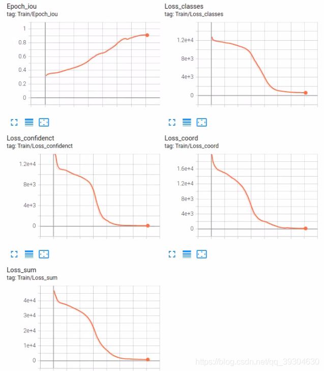
全卷积网络收敛情况
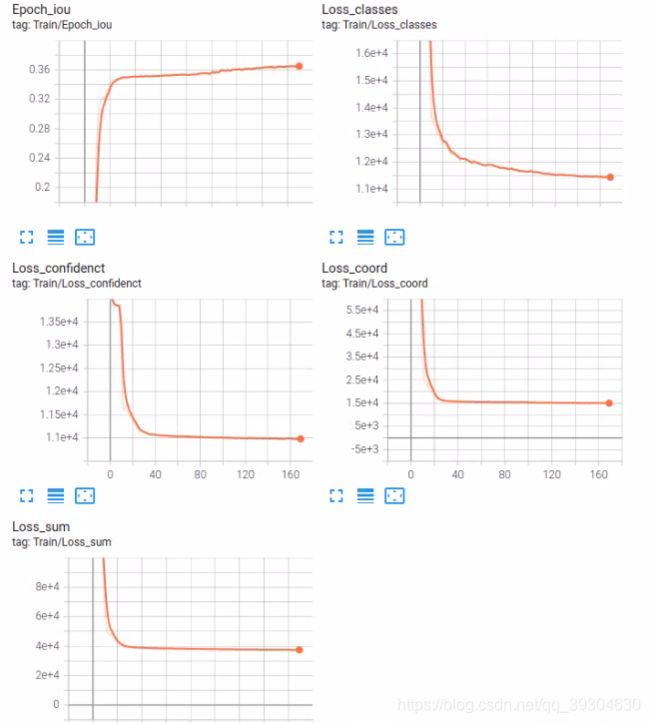
YOLO V1原网络收敛情况
项目复现github地址:https://github.com/ProgrammerZhujinming/YOLO_V1_GPU