Python可视化43|plotnine≈R语言ggplot2
- plotnine是图层图形语法(The Grammar of Graphics)在python中的实现,是ggplot2的python办,使用方法和ggplot2几乎一样。
- 本文将基于图层图形语法(The Grammar of Graphics)系统介绍plotnine,不纠结某一个具体图某一个参数,力争全局把握。
往期精彩

目录
plotnine安装
plotnine中数据集(data)
plotnine中图像属性(aesthetic attributes)
plotnine中几何对象(geometric objects)
plotnine中统计变换(statistical transformations)
plotnine中标度(scales)
plotnine中位置设置(Position adjustments)
plotnine中坐标系(coordinate system)
plotnine中分面(facet)
plotnine中主题(Themes)及子图绘制
plotnine安装
-
使用pip安装
#指定清华源快速安装plotnine
pip install plotnine -i https://pypi.tuna.tsinghua.edu.cn/simple-
使用conda安装
conda install plotnine-
linux使用git安装
git clone https://github.com/has2k1/plotnine.git
cd plotnine
pip install -e .
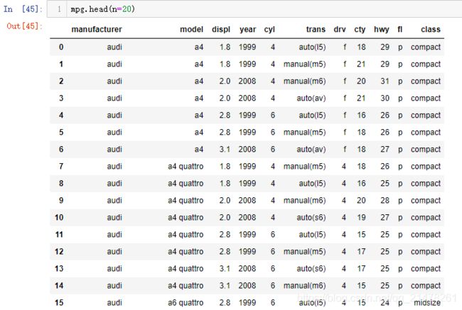
plotnine中数据集(data)
使用pandas.DataFrame类型数据集
#内置数据集
print(dir(plotnine.data))
'diamonds', 'economics', 'economics_long', 'faithful', 'faithfuld', 'huron', 'luv_colours', 'meat', 'midwest', 'mpg', 'msleep', 'mtcars', 'pageviews', 'presidential', 'seals', 'txhousing'
plotnine中图像属性(aesthetic attributes)
data to the aesthetic attributes (colour, shape, size)
#aes中设置点的属性,按class使用不同颜色
ggplot(mpg, aes('displ', 'hwy', colour = 'class')) + geom_point()
plotnine中几何对象(geometric objects)
几乎和ggplot2一样,都是以geom_开头的函数,如下:
print(len([i for i in dir(plotnine.geoms) if i.startswith('geom_')]))
print([i for i in dir(plotnine.geoms) if i.startswith('geom_')])#41中基础图
41 ['geom_abline', 'geom_area', 'geom_bar', 'geom_bin2d', 'geom_blank', 'geom_boxplot', 'geom_col', 'geom_count', 'geom_crossbar', 'geom_density', 'geom_density_2d', 'geom_dotplot', 'geom_errorbar', 'geom_errorbarh', 'geom_freqpoly', 'geom_histogram', 'geom_hline', 'geom_jitter', 'geom_label', 'geom_line', 'geom_linerange', 'geom_map', 'geom_path', 'geom_point', 'geom_pointrange', 'geom_polygon', 'geom_qq', 'geom_qq_line', 'geom_quantile', 'geom_rect', 'geom_ribbon', 'geom_rug', 'geom_segment', 'geom_sina', 'geom_smooth', 'geom_spoke', 'geom_step', 'geom_text', 'geom_tile', 'geom_violin', 'geom_vline']
ggplot(mpg, aes('class', 'hwy')) + geom_boxplot()#geom_boxplot()绘制箱图
ggplot(mpg, aes('class', 'hwy')) + geom_violin()#geom_violin()绘制小提琴图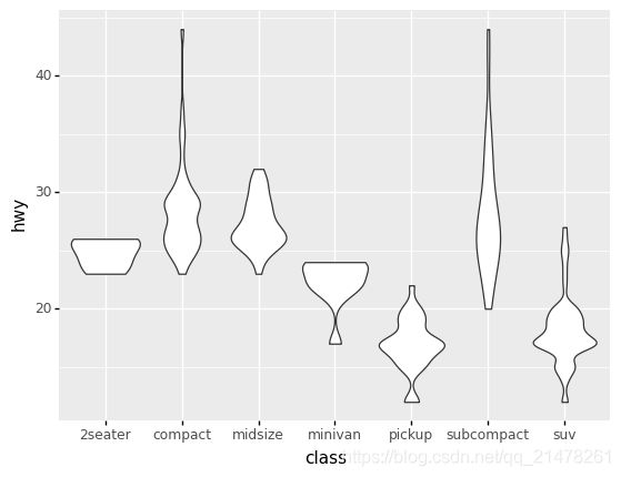
plotnine中统计变换(statistical transformations)
print([i for i in dir(plotnine.stats) if i.startswith('stat_')])['stat_bin', 'stat_bin2d', 'stat_bin_2d', 'stat_bindot', 'stat_boxplot', 'stat_count', 'stat_density', 'stat_density_2d', 'stat_ecdf', 'stat_ellipse', 'stat_function', 'stat_hull', 'stat_identity', 'stat_qq', 'stat_qq_line', 'stat_quantile', 'stat_sina', 'stat_smooth', 'stat_sum', 'stat_summary', 'stat_summary_bin', 'stat_unique', 'stat_ydensity']
#统计每组数据均值,红点表示
ggplot(mpg, aes('trans', 'cty')) + geom_boxplot() + stat_summary(
    mapping=None,
    data=None,
    geom='point',
    fun_data='mean_cl_boot',  #计算均值,这里用法与ggplot2用法有差异,help(stat_summary)查看详细用法
    colour='red',
    size=4) + \
    theme(axis_text_x = element_text(angle=90, hjust=1))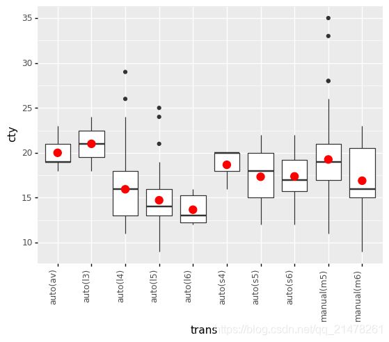
plotnine中标度(scales)
将数据取值映射到图形空间,使用颜色,形状,大小表示不同取值,使用图例,网格线展示标度,可使用的函数:
print([i for i in dir(plotnine.scales) if i.startswith('scale_')])['scale_alpha', 'scale_alpha_continuous', 'scale_alpha_datetime', 'scale_alpha_discrete', 'scale_alpha_identity', 'scale_alpha_manual', 'scale_alpha_ordinal', 'scale_color', 'scale_color_brewer', 'scale_color_cmap', 'scale_color_cmap_d', 'scale_color_continuous', 'scale_color_datetime', 'scale_color_desaturate', 'scale_color_discrete', 'scale_color_distiller', 'scale_color_gradient', 'scale_color_gradient2', 'scale_color_gradientn', 'scale_color_gray', 'scale_color_grey', 'scale_color_hue', 'scale_color_identity', 'scale_color_manual', 'scale_color_ordinal', 'scale_colour_brewer', 'scale_colour_cmap', 'scale_colour_cmap_d', 'scale_colour_continuous', 'scale_colour_datetime', 'scale_colour_desaturate', 'scale_colour_discrete', 'scale_colour_distiller', 'scale_colour_gradient', 'scale_colour_gradient2', 'scale_colour_gradientn', 'scale_colour_gray', 'scale_colour_grey', 'scale_colour_hue', 'scale_colour_identity', 'scale_colour_manual', 'scale_colour_ordinal', 'scale_fill_brewer', 'scale_fill_cmap', 'scale_fill_cmap_d', 'scale_fill_continuous', 'scale_fill_datetime', 'scale_fill_desaturate', 'scale_fill_discrete', 'scale_fill_distiller', 'scale_fill_gradient', 'scale_fill_gradient2', 'scale_fill_gradientn', 'scale_fill_gray', 'scale_fill_grey', 'scale_fill_hue', 'scale_fill_identity', 'scale_fill_manual', 'scale_fill_ordinal', 'scale_identity', 'scale_linetype', 'scale_linetype_continuous', 'scale_linetype_discrete', 'scale_linetype_identity', 'scale_linetype_manual', 'scale_manual', 'scale_shape', 'scale_shape_continuous', 'scale_shape_discrete', 'scale_shape_identity', 'scale_shape_manual', 'scale_size', 'scale_size_area', 'scale_size_continuous', 'scale_size_datetime', 'scale_size_discrete', 'scale_size_identity', 'scale_size_manual', 'scale_size_ordinal', 'scale_size_radius', 'scale_stroke', 'scale_stroke_continuous', 'scale_stroke_discrete', 'scale_x_continuous', 'scale_x_date', 'scale_x_datetime', 'scale_x_discrete', 'scale_x_log10', 'scale_x_reverse', 'scale_x_sqrt', 'scale_x_timedelta', 'scale_xy', 'scale_y_continuous', 'scale_y_date', 'scale_y_datetime', 'scale_y_discrete', 'scale_y_log10', 'scale_y_reverse', 'scale_y_sqrt', 'scale_y_timedelta']
#点按f1使用不同marker,按cty使用不同siz
ggplot(mpg, aes('displ', 'hwy', colour='class')) + geom_point(
    aes(shape='fl', size='cty')) + scale_shape() + scale_size()
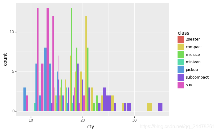
plotnine中位置设置(Position adjustments)
print([i for i in dir(plotnine.positions) if i.startswith('position_')])['position_dodge', 'position_dodge2', 'position_fill', 'position_identity', 'position_jitter', 'position_jitterdodge', 'position_nudge', 'position_stack']
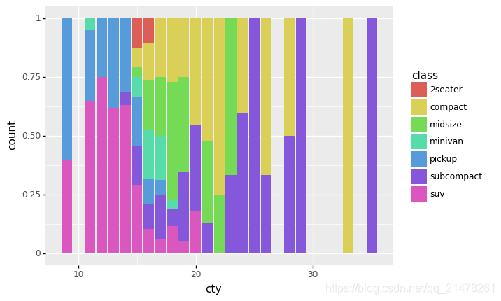
print(ggplot(mpg, aes('cty', fill='class')) + geom_bar())#堆叠barplot
print(ggplot(mpg, aes('cty', fill='class')) + geom_bar(position = "fill"))#填充barplot
print(ggplot(mpg, aes('cty', fill='class')) + geom_bar(position = "dodge"))#并列barplot
plotnine中坐标系(coordinate system)
print([i for i in dir(plotnine.coords) if i.startswith('coord_')])['coord_cartesian', 'coord_equal', 'coord_fixed', 'coord_flip', 'coord_trans']
plotnine中分面(facet)

#facet_wrap,如下
(ggplot(mpg, aes(x='displ', y='hwy'))
    + geom_point()
    + facet_wrap('class')
    + labs(x='displacement', y='horsepower'))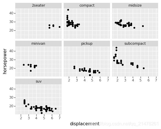
#facet_grid,如下
(
    ggplot(mpg, aes(x='displ', y='hwy'))
    + geom_point()
    + facet_grid('drv ~ .', labeller = 'label_both')
    + labs(x='displacement', y='horsepower')
)

#facet_null()单个图,不介绍
plotnine中主题(Themes)及子图绘制
print([i for i in dir(plotnine.themes) if i.startswith('theme_')])['theme_538', 'theme_bw', 'theme_classic', 'theme_dark', 'theme_get', 'theme_gray', 'theme_grey', 'theme_light', 'theme_linedraw', 'theme_matplotlib', 'theme_minimal', 'theme_seaborn', 'theme_set', 'theme_update', 'theme_void', 'theme_xkcd']
from matplotlib import gridspec
p1 = ggplot(mpg, aes('displ', 'hwy')) + geom_point() + geom_smooth() + theme_xkcd()
p2 = ggplot(mpg, aes('displ', 'hwy')) + geom_point() + geom_smooth() + coord_cartesian(xlim=(5, 7)) + theme_dark()
p3 = ggplot(mpg, aes('cty', 'displ')) + geom_point() + geom_smooth() +theme_matplotlib()
p4 = ggplot(mpg, aes('displ', 'cty')) +  geom_point() + geom_smooth() +  coord_fixed() + theme_linedraw()

# 绘制多子图
fig = (ggplot()+geom_blank(data=mpg)+theme_void()).draw()
gs = gridspec.GridSpec(2,2)
ax1 = fig.add_subplot(gs[0,0])
ax2 = fig.add_subplot(gs[0,1])
ax3 = fig.add_subplot(gs[1,0])
ax4 = fig.add_subplot(gs[1,1])
_ = p1._draw_using_figure(fig,[ax1])
_ = p2._draw_using_figure(fig,[ax2])
_ = p3._draw_using_figure(fig,[ax3])
_ = p4._draw_using_figure(fig,[ax4])
plt.tight_layout()
plt.show() 
参考资料:https://plotnine.readthedocs.io/en/stable/#
