使用SnapATAC分析单细胞ATAC-seq数据（三）：Integrative Analysis of PBMC scATAC-seq and scRNA-seq

image.png

简介

在本教程中，我们将对PBMC的两个scATAC-seq数据集(5K和10K)和一个scRNA-seq数据集进行整合分析。这三个数据集均来自10X genomics测序平台产生的数据，可以直接在10x官网下载使用。
具体来说，我们将主要执行以下分析内容：

• Cell selection for PBMC 5k and 10k scATAC;
• Randomly sample 10,000 cells as landmarks;
• Unsupervised clustering of landmarks;
• Project the remaining (query) cells onto the landmarks;
• Supervised annotation of scATAC clusters using scRNA dataset;
• Downstream analysis including peak calling, differential analysis, prediction of gene-enhancer pairing.

分析步骤

• Step 0. Data download
• Step 1. Barcode selection
• Step 2. Add cell-by-bin matrix
• Step 3. Matrix binarization
• Step 4. Bin filtering
• Step 5. Dimensionality reduction of landmarks
• Step 6. Determine significant components
• Step 7. Graph-based clustering
• Step 8. Visualization
• Step 9. scRNA-seq based annotation
• Step 10. Create psudo multiomics cells
• Step 11. Remove cells of low prediction score
• Step 12. Gene expression projected into UMAP
• Step 13. Identify peak
• Step 14. Create a cell-by-peak matrix
• Step 15. Identify differentially accessible regions
• Step 16. Motif variability analysis
• Step 17. De novo motif discovery
• Step 18. Predict gene-enhancer pairs

Step 0. Data Download

开始分析之前，我们需要下载snaptools生成的snap文件和cellranger-atac产生的singlecell.csv文件。

# 下载所需的数据集和基因注释信息
$ wget http://renlab.sdsc.edu/r3fang//share/github/PBMC_ATAC_RNA/atac_pbmc_5k_nextgem.snap
$ wget http://cf.10xgenomics.com/samples/cell-atac/1.1.0/atac_pbmc_5k_nextgem/atac_pbmc_5k_nextgem_singlecell.csv
$ wget http://renlab.sdsc.edu/r3fang//share/github/PBMC_ATAC_RNA/atac_pbmc_10k_nextgem.snap
$ wget http://cf.10xgenomics.com/samples/cell-atac/1.1.0/atac_pbmc_10k_nextgem/atac_pbmc_10k_nextgem_singlecell.csv
$ wget http://cf.10xgenomics.com/samples/cell-atac/1.1.0/atac_pbmc_10k_nextgem/hg19.blacklist.bed.gz
$ wget http://cf.10xgenomics.com/samples/cell-atac/1.1.0/gencode.v19.annotation.gene.bed

Step 1. Barcode selection

首先，我们根据以下两个主要的标准来选择高质量的barcodes：

1. number of unique fragments;
2. fragments in promoter ratio;

# 加载所需R包
> library(SnapATAC);
> snap.files = c(
    "atac_pbmc_5k_nextgem.snap", 
    "atac_pbmc_10k_nextgem.snap"
  );
> sample.names = c(
    "PBMC 5K",
    "PBMC 10K"
  );
> barcode.files = c(
    "atac_pbmc_5k_nextgem_singlecell.csv",
    "atac_pbmc_10k_nextgem_singlecell.csv"
  );

# 读取snap文件
> x.sp.ls = lapply(seq(snap.files), function(i){
    createSnap(
        file=snap.files[i],
        sample=sample.names[i]
    );
  })
> names(x.sp.ls) = sample.names;

# 读取barcode信息
> barcode.ls = lapply(seq(snap.files), function(i){
    barcodes = read.csv(
        barcode.files[i], 
        head=TRUE
    );
    # remove NO BAROCDE line
    barcodes = barcodes[2:nrow(barcodes),];
    barcodes$logUMI = log10(barcodes$passed_filters + 1);
    barcodes$promoter_ratio = (barcodes$promoter_region_fragments+1) / (barcodes$passed_filters + 1);
    barcodes
  })

# 质控指标数据可视化
> plots = lapply(seq(snap.files), function(i){
    p1 = ggplot(
        barcode.ls[[i]], 
        aes(x=logUMI, y=promoter_ratio)) + 
        geom_point(size=0.3, col="grey") +
        theme_classic() +
        ggtitle(sample.names[[i]]) +
        ylim(0, 1) + xlim(0, 6) + 
        labs(x = "log10(UMI)", y="promoter ratio")
        p1
    })
> plots

image.png

# 查看snap对象信息
> x.sp.ls
## $`PBMC 5K`
## number of barcodes: 20000
## number of bins: 0
## number of genes: 0
## number of peaks: 0
## number of motifs: 0
## 
## $`PBMC 10K`
## number of barcodes: 20000
## number of bins: 0
## number of genes: 0
## number of peaks: 0
## number of motifs: 0

# for both datasets, we identify usable barcodes using [3.5-5] for log10(UMI) and [0.4-0.8] for promoter ratio as cutoff.
# 设定质控阈值进行筛选过滤
> cutoff.logUMI.low = c(3.5, 3.5);
> cutoff.logUMI.high = c(5, 5);
> cutoff.FRIP.low = c(0.4, 0.4);
> cutoff.FRIP.high = c(0.8, 0.8);

# 根据过滤的阈值进行barcode的筛选
> barcode.ls = lapply(seq(snap.files), function(i){
    barcodes = barcode.ls[[i]];
    idx = which(
        barcodes$logUMI >= cutoff.logUMI.low[i] & 
        barcodes$logUMI <= cutoff.logUMI.high[i] & 
        barcodes$promoter_ratio >= cutoff.FRIP.low[i] &
        barcodes$promoter_ratio <= cutoff.FRIP.high[i]
    );
    barcodes[idx,]
  });

> x.sp.ls = lapply(seq(snap.files), function(i){
    barcodes = barcode.ls[[i]];
    x.sp = x.sp.ls[[i]];
    barcode.shared = intersect(x.sp@barcode, barcodes$barcode);
    x.sp = x.sp[match(barcode.shared, x.sp@barcode),];
    barcodes = barcodes[match(barcode.shared, barcodes$barcode),];
    x.sp@metaData = barcodes;
    x.sp
  })

> names(x.sp.ls) = sample.names;
> x.sp.ls
## $`PBMC 5K`
## number of barcodes: 4526
## number of bins: 0
## number of genes: 0
## number of peaks: 0
## number of motifs: 0
## 
## $`PBMC 10K`
## number of barcodes: 9039
## number of bins: 0
## number of genes: 0
## number of peaks: 0
## number of motifs: 0
# combine two snap object

# combine two snap object
# 使用Reduce函数将两个snap对象进行合并
> x.sp = Reduce(snapRbind, x.sp.ls);
> x.sp@metaData["sample"] = x.sp@sample;

> x.sp
## number of barcodes: 13565
## number of bins: 0
## number of genes: 0
## number of peaks: 0

> table(x.sp@sample);
## PBMC 10K  PBMC 5K
##     9039     4526

Step 2. Add cell-by-bin matrix

接下来，我们使用addBmatToSnap函数生成5kb分辨率的cell-by-bin计数矩阵，并将其添加到snap对象中。该函数将自动从两个snap文件中读取cell-by-bin矩阵，并将连接后的矩阵添加到snap对象的bmat属性中。

# 使用addBmatToSnap函数计算cell-by-bin计数矩阵
> x.sp = addBmatToSnap(x.sp, bin.size=5000);

Step 3. Matrix binarization

我们使用makeBinary函数将cell-by-bin计数矩阵转换为二进制矩阵。在count矩阵中，某些项具有异常高的覆盖率，这可能是由比对错误造成的。因此，我们将删除计数矩阵中top 0.1%的项，并将其余非零的值转换为1。

# 使用makeBinary函数将cell-by-bin计数矩阵转换成二进制矩阵
> x.sp = makeBinary(x.sp, mat="bmat");

Step 4. Bin filtering

首先，我们过滤掉任何与ENCODE中blacklist区域重叠的bins，以防止潜在的artifacts。

> library(GenomicRanges);
# 读取blacklist信息
> black_list = read.table("hg19.blacklist.bed.gz");
> black_list.gr = GRanges(
    black_list[,1], 
    IRanges(black_list[,2], black_list[,3])
  );

> idy = queryHits(
    findOverlaps(x.sp@feature, black_list.gr)
  );
> if(length(idy) > 0){
    x.sp = x.sp[,-idy, mat="bmat"];
  };
> x.sp
## number of barcodes: 13565
## number of bins: 624794
## number of genes: 0
## number of peaks: 0
## number of motifs: 0

接下来，我们移除那些不需要的染色体信息。

> chr.exclude = seqlevels(x.sp@feature)[grep("random|chrM", seqlevels(x.sp@feature))];

> idy = grep(paste(chr.exclude, collapse="|"), x.sp@feature);
> if(length(idy) > 0){
    x.sp = x.sp[,-idy, mat="bmat"]
  };
> x.sp
## number of barcodes: 13565
## number of bins: 624297
## number of genes: 0
## number of peaks: 0
## number of motifs: 0

第三，bins的覆盖率大致是服从对数正态分布的。我们将与不变特征(如管家基因的启动子)重叠的前5%的bins进行删除 。

> bin.cov = log10(Matrix::colSums(x.sp@bmat)+1);
> hist(
    bin.cov[bin.cov > 0], 
    xlab="log10(bin cov)", 
    main="log10(Bin Cov)", 
    col="lightblue", 
    xlim=c(0, 5)
  );
> bin.cutoff = quantile(bin.cov[bin.cov > 0], 0.95);
> idy = which(bin.cov <= bin.cutoff & bin.cov > 0);
> x.sp = x.sp[, idy, mat="bmat"];
> x.sp
## number of barcodes: 13565
## number of bins: 534985
## number of genes: 0
## number of peaks: 0
## number of motifs: 0

image.png

最后，我们将进一步删除bin覆盖率小于1000的任何细胞，这是因为尽管有些细胞可能含有较高的unique fragments片段，但是过滤后的bin覆盖率却很低。此步骤是可选的，但强烈建议这样做。

> idx = which(Matrix::rowSums(x.sp@bmat) > 1000);
> x.sp = x.sp[idx,];
> x.sp
## number of barcodes: 13434
## number of bins: 534985
## number of genes: 0
## number of peaks: 0
## number of motifs: 0

Step 5. Dimentionality reduction

SnapATAC采用diffusion maps算法进行数据降维，这是一种非线性降维的技术，它通过对数据执行random walk来发现低维的manifold，并且对噪音和扰动具有很强的鲁棒性。

但是，diffusion maps算法的计算成本会随着细胞数目的增加而呈现指数级增长的趋势。为了克服这一局限，我们将Nyström方法(a sampling technique)和diffusion maps算法相结合，给出Nyström Landmark diffusion map来生成大规模数据集的低维嵌入。

Nyström landmark diffusion maps算法主要包括以下三个步骤：

• sampling: sample a subset of K (K≪N) cells from N total cells as “landmarks”. Instead of random sampling, here we adopted a density-based sampling approach developed in SCTransform to preserve the density distribution of the N original points;
• embedding: compute a diffusion map embedding for K landmarks;
• extension: project the remaining N-K cells onto the low-dimensional embedding as learned from the landmarks to create a joint embedding space for all cells.

在本示例中，我们将采样10,000个细胞作为landmarks，并将余下的query细胞投射到嵌入landmarks的diffusion maps上。

> row.covs.dens <- density(
    x = x.sp@metaData[,"logUMI"], 
    bw = 'nrd', adjust = 1
  );
> sampling_prob <- 1 / (approx(x = row.covs.dens$x, y = row.covs.dens$y, xout = x.sp@metaData[,"logUMI"])$y + .Machine$double.eps);

> set.seed(1);
> idx.landmark.ds <- sort(sample(x = seq(nrow(x.sp)), size = 10000, prob = sampling_prob));

将x.sp对象分割为landmark(x.landmark.sp)细胞和query(x.query.sp)细胞。

> x.landmark.sp = x.sp[idx.landmark.ds,];
> x.query.sp = x.sp[-idx.landmark.ds,];

Run diffusion maps on the landmark cells.
使用landmark细胞进行diffusion maps降维处理

> x.landmark.sp = runDiffusionMaps(
    obj= x.landmark.sp,
    input.mat="bmat", 
    num.eigs=50
  );
> x.landmark.sp@metaData$landmark = 1;

Porject query cells to landmarks.
将query细胞映射到landmarks上

> x.query.sp = runDiffusionMapsExtension(
    obj1=x.landmark.sp, 
    obj2=x.query.sp,
    input.mat="bmat"
  );
> x.query.sp@metaData$landmark = 0;

Combine landmark and query cells.
合并landmark和query细胞
Note: To merge snap objects, all the matrix (bmat, gmat, pmat) and metaData must be of the same number of columns between snap objects.

> x.sp = snapRbind(x.landmark.sp, x.query.sp);
> x.sp = x.sp[order(x.sp@metaData[,"sample"])]; #IMPORTANT

Step 6. Determine significant components

接下来，我们将确定特征向量（eigen-vectors）的数目，以便用于后续的分析。在下面的例子中，我们选择前15个特征向量。

> plotDimReductPW(
    obj=x.sp, 
    eigs.dims=1:50,
    point.size=0.3,
    point.color="grey",
    point.shape=19,
    point.alpha=0.6,
    down.sample=5000,
    pdf.file.name=NULL, 
    pdf.height=7, 
    pdf.width=7
  );

image.png

Step 7. Graph-based clustering

接下来，我们使用所选的特征向量成分，来构造K近邻（KNN）聚类图。其中，每个节点是一个细胞，根据欧氏距离来确定每个细胞的k个近邻细胞。

> x.sp = runKNN(
    obj=x.sp,
    eigs.dims=1:20,
    k=15
  );

> library(leiden);
> x.sp=runCluster(
    obj=x.sp,
    tmp.folder=tempdir(),
    louvain.lib="leiden",
    seed.use=10,
    resolution=0.7
  );

Step 8. Visualization

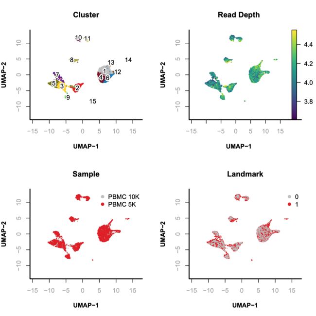
SnapATAC可以使用tSNE(FI-tsne)和UMAP方法对降维聚类后的细胞进行可视化的展示和探索。在本示例中，我们使用UMAP方法进行展示。

> library(umap);
> x.sp = runViz(
    obj=x.sp, 
    tmp.folder=tempdir(),
    dims=2,
    eigs.dims=1:20, 
    method="umap",
    seed.use=10
  );

> par(mfrow = c(2, 2));
> plotViz(
    obj= x.sp,
    method="umap", 
    main="Cluster",
    point.color=x.sp@cluster, 
    point.size=0.2, 
    point.shape=19, 
    text.add=TRUE,
    text.size=1,
    text.color="black",
    down.sample=10000,
    legend.add=FALSE
  );
> plotFeatureSingle(
    obj=x.sp,
    feature.value=x.sp@metaData[,"logUMI"],
    method="umap", 
    main="Read Depth",
    point.size=0.2, 
    point.shape=19, 
    down.sample=10000,
    quantiles=c(0.01, 0.99)
  );
> plotViz(
    obj= x.sp,
    method="umap", 
    main="Sample",
    point.size=0.2, 
    point.shape=19, 
    point.color=x.sp@sample, 
    text.add=FALSE,
    text.size=1.5,
    text.color="black",
    down.sample=10000,
    legend.add=TRUE
    );
> plotViz(
    obj= x.sp,
    method="umap", 
    main="Landmark",
    point.size=0.2, 
    point.shape=19, 
    point.color=x.sp@metaData[,"landmark"], 
    text.add=FALSE,
    text.size=1.5,
    text.color="black",
    down.sample=10000,
    legend.add=TRUE
  );

image.png

Step 9. scRNA-seq based annotation

在本示例中，我们将使用相应的scRNA-seq数据集来对scATAC-seq数据的细胞类群进行注释。我们可以通过(https://www.dropbox.com/s/3f3p5nxrn5b3y4y/pbmc_10k_v3.rds?dl=1)地址下载所需的10X PBMC scRNA-seq(pbmc_10k_v3.rds)的Seurat对象。

> library(Seurat);
> pbmc.rna = readRDS("pbmc_10k_v3.rds");
> pbmc.rna$tech = "rna";
> variable.genes = VariableFeatures(object = pbmc.rna);

> genes.df = read.table("gencode.v19.annotation.gene.bed");
> genes.gr = GRanges(genes.df[,1], IRanges(genes.df[,2], genes.df[,3]), name=genes.df[,4]);
> genes.sel.gr = genes.gr[which(genes.gr$name %in% variable.genes)];

## reload the bmat, this is optional but highly recommanded
> x.sp = addBmatToSnap(x.sp);
> x.sp = createGmatFromMat(
    obj=x.sp, 
    input.mat="bmat",
    genes=genes.sel.gr,
    do.par=TRUE,
    num.cores=10
  );

接下来，我们将snap对象转换为Seurat对象，用于后续的数据整合。

# 使用snapToSeurat函数将snap对象转换为Seurat对象
> pbmc.atac <- snapToSeurat(
    obj=x.sp, 
    eigs.dims=1:20, 
    norm=TRUE,
    scale=TRUE
  );

# 识别整合的Anchors信息
> transfer.anchors <- FindTransferAnchors(
    reference = pbmc.rna, 
    query = pbmc.atac, 
    features = variable.genes, 
    reference.assay = "RNA", 
    query.assay = "ACTIVITY", 
    reduction = "cca"
  );

# 使用TransferData函数进行数据映射整合
> celltype.predictions <- TransferData(
    anchorset = transfer.anchors, 
    refdata = pbmc.rna$celltype,
    weight.reduction = pbmc.atac[["SnapATAC"]],
    dims = 1:20
  );
> x.sp@metaData$predicted.id = celltype.predictions$predicted.id;
> x.sp@metaData$predict.max.score = apply(celltype.predictions[,-1], 1, max);
> x.sp@cluster = as.factor(x.sp@metaData$predicted.id);

Step 10. Create psudo multiomics cells

现在，snap对象x.sp中包含了的每个细胞的染色质可及性@bmat和基因表达@gmat的信息。

> refdata <- GetAssayData(
    object = pbmc.rna, 
    assay = "RNA", 
    slot = "data"
  );
> imputation <- TransferData(
    anchorset = transfer.anchors, 
    refdata = refdata, 
    weight.reduction = pbmc.atac[["SnapATAC"]], 
    dims = 1:20
  );
> x.sp@gmat = t(imputation@data);
> rm(imputation); # free memory
> rm(refdata);    # free memory
> rm(pbmc.rna);   # free memory
> rm(pbmc.atac); # free memory

Step 11. Remove cells of low prediction score

> hist(
    x.sp@metaData$predict.max.score, 
    xlab="prediction score", 
    col="lightblue", 
    xlim=c(0, 1),
    main="PBMC 10X"
  );
> abline(v=0.5, col="red", lwd=2, lty=2);

> table(x.sp@metaData$predict.max.score > 0.5);
## FALSE  TRUE
##  331 13103

> x.sp = x.sp[x.sp@metaData$predict.max.score > 0.5,];
> x.sp
## number of barcodes: 13045
## number of bins: 627478
## number of genes: 19089
## number of peaks: 0

> plotViz(
    obj=x.sp,
    method="umap", 
    main="PBMC 10X",
    point.color=x.sp@metaData[,"predicted.id"], 
    point.size=0.5, 
    point.shape=19, 
    text.add=TRUE,
    text.size=1,
    text.color="black",
    down.sample=10000,
    legend.add=FALSE
  );

image.png

Step 12. Gene expression projected onto UMAP

接下来，我们使用UMAP方法对一些marker基因的表达水平进行可视化展示。

> marker.genes = c(
    "IL32", "LTB", "CD3D",
    "IL7R", "LDHB", "FCGR3A", 
    "CD68", "MS4A1", "GNLY", 
    "CD3E", "CD14", "CD14", 
    "FCGR3A", "LYZ", "PPBP", 
    "CD8A", "PPBP", "CST3", 
    "NKG7", "MS4A7", "MS4A1", 
    "CD8A"
  );

> par(mfrow = c(3, 3));
> for(i in 1:9){
    j = which(colnames(x.sp@gmat) == marker.genes[i])
    plotFeatureSingle(
        obj=x.sp,
        feature.value=x.sp@gmat[,j],
        method="umap", 
        main=marker.genes[i],
        point.size=0.1, 
        point.shape=19, 
        down.sample=10000,
        quantiles=c(0.01, 0.99)
 )};

image.png

Step 13. Identify peaks

接下来，我们将每个cluster群中的reads进行聚合，创建用于peak calling和可视化的集成track。执行完peak calling后，将生成一个.narrowPeak的文件，该文件中包含了识别出的peaks信息，和一个.bedgraph的文件，可以用于可视化展示。为了获得最robust的结果，我们不建议对细胞数目小于100的cluster群执行此步骤。

> system("which snaptools");
/home/r3fang/anaconda2/bin/snaptools
> system("which macs2");
/home/r3fang/anaconda2/bin/macs2

# 使用runMACS函数调用macs2进行peak calling
> peaks = runMACS(
    obj=x.sp[which(x.sp@cluster=="CD4 Naive"),], 
    output.prefix="PBMC.CD4_Naive",
    path.to.snaptools="/home/r3fang/anaconda2/bin/snaptools",
    path.to.macs="/home/r3fang/anaconda2/bin/macs2",
    gsize="hs", # mm, hs, etc
    buffer.size=500, 
    num.cores=10,
    macs.options="--nomodel --shift 100 --ext 200 --qval 5e-2 -B --SPMR",
    tmp.folder=tempdir()
    );

为了对所有的cluster群执行peak calling，我们提供了一个简便的脚本来实现该步骤。

# call peaks for all cluster with more than 100 cells
# 选出那些细胞数目大于100的cluster群
> clusters.sel = names(table(x.sp@cluster))[which(table(x.sp@cluster) > 100)];

# 批量对不同的cluster进行peak calling
> peaks.ls = mclapply(seq(clusters.sel), function(i){
    print(clusters.sel[i]);
    peaks = runMACS(
        obj=x.sp[which(x.sp@cluster==clusters.sel[i]),], 
        output.prefix=paste0("PBMC.", gsub(" ", "_", clusters.sel)[i]),
        path.to.snaptools="/home/r3fang/anaconda2/bin/snaptools",
        path.to.macs="/home/r3fang/anaconda2/bin/macs2",
        gsize="hs", # mm, hs, etc
        buffer.size=500, 
        num.cores=1,
        macs.options="--nomodel --shift 100 --ext 200 --qval 5e-2 -B --SPMR",
        tmp.folder=tempdir()
   );
    peaks
    }, mc.cores=5);

> peaks.names = system("ls | grep narrowPeak", intern=TRUE);

> peak.gr.ls = lapply(peaks.names, function(x){
    peak.df = read.table(x)
    GRanges(peak.df[,1], IRanges(peak.df[,2], peak.df[,3]))
  })

# 合并peak信息
> peak.gr = reduce(Reduce(c, peak.gr.ls));

我们可以将每个cluster群生成的bdg文件导入到IGV或其他基因组浏览器(如UW genome browser)进行可视化的展示，下面是来自UW genome browser的FOXJ2基因及其侧翼区域的screenshot。

image.png

Step 14. Create a cell-by-peak matrix

接下来，我们使用合并后的peaks作为参考，来创建一个cell-by-peak计数矩阵，并将其添加到snap对象中。
首先，我们将合并后的peaks信息写入到peaks.combined.bed文件中

> peaks.df = as.data.frame(peak.gr)[,1:3];
> write.table(peaks.df,file = "peaks.combined.bed",append=FALSE,
        quote= FALSE,sep="\t", eol = "\n", na = "NA", dec = ".", 
        row.names = FALSE, col.names = FALSE, qmethod = c("escape", "double"),
        fileEncoding = "")

接下来，我们创建一个cell-by-peak计数矩阵，并将其添加到snap对象中。这一步可能需要一段时间。

$ snaptools snap-add-pmat \
    --snap-file atac_pbmc_10k_nextgem.snap \
    --peak-file peaks.combined.bed &
$ snaptools snap-add-pmat \
    --snap-file atac_pbmc_5k_nextgem.snap \
    --peak-file peaks.combined.bed  

然后，我们将计算好的cell-by-peak计数矩阵添加到已有的snap对象中。

> x.sp = addPmatToSnap(x.sp);

Step 15. Identify differentially accessible peaks

对于一组给定的细胞Ci，我们首先在diffusion component空间中寻找邻近的细胞Cj (|Ci|=|Cj|)作为“background”细胞进行比较。如果Ci细胞的数目占总细胞数目的一半以上，则使用剩余的细胞作为local background。接下来，我们将Ci和Cj细胞进行聚合，来创建两个raw-count向量，即Vci和Vcj。然后，我们使用R包edgeR (v3.18.1)的精确检验（exact test）来对Vci和Vcj进行差异分析，其中，对于小鼠设置BCV=0.1，而人类设置BCV= 0.4。最后，再使用Benjamini-Hochberg多重检验校正方法，来调整p-value值为错误发现率(FDR)值。对于FDR值小于0.05的peaks，被选为显著的DARs。

我们发现这种方法也存在一定的局限性，特别是对于那些细胞数目较少的cluster群，统计的有效性可能不够强大。对于那些未能识别出显著差异peaks的cluster群，我们将根据富集p-value值对元素进行排序，并挑选出最具代表性的2,000个peaks进行后续的motif分析。

> DARs = findDAR(
    obj=x.sp,
    input.mat="pmat",
    cluster.pos="CD14+ Monocytes",
    cluster.neg.method="knn",
    test.method="exactTest",
    bcv=0.4, #0.4 for human, 0.1 for mouse
    seed.use=10
  );
> DARs$FDR = p.adjust(DARs$PValue, method="BH");
> idy = which(DARs$FDR < 5e-2 & DARs$logFC > 0);

> par(mfrow = c(1, 2));
> plot(DARs$logCPM, DARs$logFC, 
    pch=19, cex=0.1, col="grey", 
    ylab="logFC", xlab="logCPM",
    main="CD14+ Monocytes"
  );
> points(DARs$logCPM[idy], 
    DARs$logFC[idy], 
    pch=19, 
    cex=0.5, 
    col="red"
  );
> abline(h = 0, lwd=1, lty=2);

> covs = Matrix::rowSums(x.sp@pmat);
> vals = Matrix::rowSums(x.sp@pmat[,idy]) / covs;
> vals.zscore = (vals - mean(vals)) / sd(vals);

> plotFeatureSingle(
    obj=x.sp,
    feature.value=vals.zscore,
    method="umap", 
    main="CD14+ Monocytes",
    point.size=0.1, 
    point.shape=19, 
    down.sample=5000,
    quantiles=c(0.01, 0.99)
  );

Step 16. Motif variability analysis

SnapATAC可以调用chromVAR(Schep et al)程序进行motif可变性分析。

# 加载所需的R包
> library(chromVAR);
> library(motifmatchr);
> library(SummarizedExperiment);
> library(BSgenome.Hsapiens.UCSC.hg19);

> x.sp = makeBinary(x.sp, "pmat");

# 使用runChromVAR函数调用ChromVAR进行motif可变性分析
> x.sp@mmat = runChromVAR(
    obj=x.sp,
    input.mat="pmat",
    genome=BSgenome.Hsapiens.UCSC.hg19,
    min.count=10,
    species="Homo sapiens"
  );
> x.sp;
## number of barcodes: 13103
## number of bins: 627478
## number of genes: 19089
## number of peaks: 157750
## number of motifs: 271

> motif_i = "MA0071.1_RORA";
> dat = data.frame(x=x.sp@metaData$predicted.id, y=x.sp@mmat[,motif_i]);
> p <- ggplot(dat, aes(x=x, y=y, fill=x)) + 
    theme_classic() +
    geom_violin() + 
    xlab("cluster") +
    ylab("motif enrichment") + 
    ggtitle("MA0071.1_RORA") +
    theme(
          plot.margin = margin(5,1,5,1, "cm"),
          axis.text.x = element_text(angle = 90, hjust = 1),
          axis.ticks.x=element_blank(),
          legend.position = "none"
   );

image.png

Step 17. De novo motif discovery

SnapATAC还可以调用homer用于对识别出的差异可及性区域(DARs)进行motif的识别和富集分析.

# 查看findMotifsGenome.pl程序安装的路径
> system("which findMotifsGenome.pl");
/projects/ps-renlab/r3fang/public_html/softwares/homer/bin/findMotifsGenome.pl

# 使用findDAR函数鉴定DAR区域
> DARs = findDAR(
    obj=x.sp,
    input.mat="pmat",
    cluster.pos="Double negative T cell",
    cluster.neg.method="knn",
    test.method="exactTest",
    bcv=0.4, #0.4 for human, 0.1 for mouse
    seed.use=10
  );
> DARs$FDR = p.adjust(DARs$PValue, method="BH");
> idy = which(DARs$FDR < 5e-2 & DARs$logFC > 0);

# 使用runHomer函数调用homer进行de novo motif discovery
> motifs = runHomer(
    x.sp[,idy,"pmat"], 
    mat = "pmat",
    path.to.homer = "/projects/ps-renlab/r3fang/public_html/softwares/homer/bin/findMotifsGenome.pl",
    result.dir = "./homer/DoubleNegativeTcell",
    num.cores=5,
    genome = 'hg19',
    motif.length = 10,
    scan.size = 300,
    optimize.count = 2,
    background = 'automatic',
    local.background = FALSE,
    only.known = TRUE,
    only.denovo = FALSE,
    fdr.num = 5,
    cache = 100,
    overwrite = TRUE,
    keep.minimal = FALSE
    );

image.png

Step 18. Predict gene-enhancer pairs

最后，我们还可以使用一种“pseudo”细胞的方法，根据单个细胞中基因的表达和远端调控元件的染色质可及性的关系，将远端调控元件连接到目标基因上。对于给定的marker基因，我们首先识别出marker基因侧翼区域内的peak。对于每个侧翼的peak，我们使用基因表达作为输入变量进行逻辑回归来预测binarized的染色质状态。产生的结果估计了染色质可及性与基因表达之间联系的重要性。

> TSS.loci = GRanges("chr12", IRanges(8219067, 8219068));

> pairs = predictGenePeakPair(
    x.sp, 
    input.mat="pmat",
    gene.name="C3AR1", 
    gene.loci=resize(TSS.loci, width=500000, fix="center"),
    do.par=FALSE
    );

# convert the pair to genome browser arc plot format
> pairs.df = as.data.frame(pairs);
> pairs.df = data.frame(
    chr1=pairs.df[,"seqnames"],
    start1=pairs.df[,"start"],
    end1=pairs.df[,"end"],
    chr2="chr2",
    start2=8219067,
    end2=8219068,
    Pval=pairs.df[,"logPval"]
    );
> head(pairs.df)
##    chr1  start1    end1 chr2  start2    end2       Pval
## 1 chr12 7984734 7985229 chr2 8219067 8219068 14.6075918
## 2 chr12 7987561 7988085 chr2 8219067 8219068  5.6718381
## 3 chr12 7989776 7990567 chr2 8219067 8219068 24.2564608
## 4 chr12 7996454 7996667 chr2 8219067 8219068  0.6411017
## 5 chr12 8000059 8000667 chr2 8219067 8219068  2.0324922
## 6 chr12 8012404 8013040 chr2 8219067 8219068  0.0000000

image.png

参考来源：https://gitee.com/booew/SnapATAC/blob/master/examples/10X_PBMC_15K/README.md