TensorFlow2.0入门到进阶系列——3_TensorFlow基础API

先上图，后改思维导图

1 @tf.function

• 将python函数编译成tf的图结构（eg:if、for、while、break、print、递归调用、列表方法等）
• 易于将python写的模型导出为GraphDef + checkpoint或者SavedModel
• 使用eager execution可以默认打开
• 1.0的代码可以通过tf.function来继续在2.0里使用
  • 2.0中的 tf.function相当于对tf1.0中的session的替代

1.1 API列表

• 基础数据类型
  • Tf.constant, tf.string
  • tf.ragged.constant, tf.SparseTensor, Tf.Variable
• 自定义损失函数——Tf.reduce_mean
• 自定义层次——Keras.layers.Lambda和继承法
• Tf.function
  • Tf.function, tf.autograph.to_code, get_concrete_function
• GraphDef
  • get_operations, get_operation_by_name
  • get_tensor_by_name, as_graph_def
• 自动求导
  • Tf.GradientTape
  • Optimzier.apply_gradients

1.2 基础API

加载库

import matplotlib as mpl
import matplotlib.pyplot as plt
%matplotlib inline
import numpy as np
import sklearn
import pandas as pd
import os
import sys
import time
import tensorflow as tf
from tensorflow import keras
#import keras

print(tf.__version__)
print(sys.version_info)
for module in mpl,np,pd,sklearn,tf,keras:
    print(module.__name__,module.__version__)

基础API

#tf第一个基础API   常量
t = tf.constant([[1.,2.,3.],[4.,5.,6.]])

#索引操作
print(t)
print(t[:,1:])
print(t[...,1])   #只得到第二列  结果是一个向量

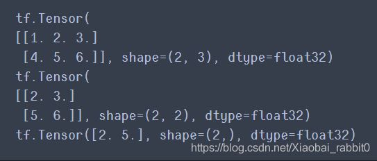
#做算子操作ops
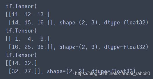
print(t + 10)      #相加
print(tf.square(t))    #平方
print(t @ tf.transpose(t))   #矩阵乘以自身的转置

#tf对象与numpy转换
print(t.numpy())     #调用numpy把值取出来
print(np.square(t)) #tf作为numpy方法的输入
#将numpy对象直接转换为tf_tensor
np_t = np.array([[1.,2.,3.],[4.,5.,6.]])       
print(tf.constant(np_t))

#Scalars
t = tf.constant(2.717)
print(t.numpy())
print(t.shape)

#strings
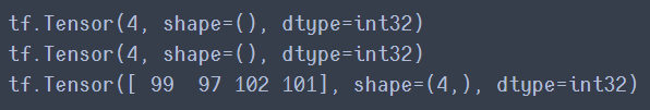
t = tf.constant("cafe")
print(tf.strings.length(t))
print(tf.strings.length(t,unit = "UTF8_CHAR"))
print(tf.strings.unicode_decode(t,"UTF8"))

#存储数组字符串 string array
#string array
t = tf.constant(["cafe","coffee","咖啡"])
print(tf.strings.length(t,unit = "UTF8_CHAR"))
r = tf.strings.unicode_decode(t,"UTF8")
print(r)

RaggedTensor不完整的矩阵

#RaggedTensor不完整的矩阵
#ragged tensor   的使用
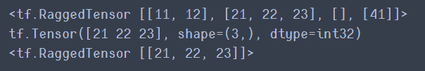
r = tf.ragged.constant([[11,12],[21,22,23],[],[41]])
# index op
print(r)
print(r[1])
print(r[1:2])

# ops on ragged tensor
#拼接操作
r2 = tf.ragged.constant([[51,52],[],[71]])
print(tf.concat([r,r2],axis = 0))    #按行拼接，第零维度

#因为行数不一致，所以按列拼接需要让其行维度相同
r3 = tf.ragged.constant([[13,14],[15],[],[42,43]])
print(tf.concat([r,r3],axis = 1))    #按列拼接

#raggedtensor  可以  变成普通tensor
print(r.to_tensor())

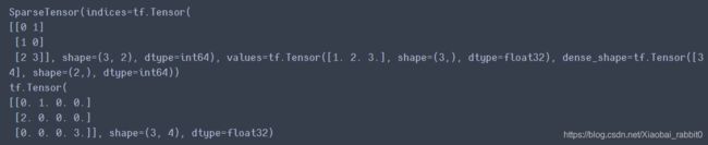
# sparse tensor
#如果一个矩阵中大部分都是0只有小部分是1，那么就可以把对应是1的值和坐标记录下来
s = tf.SparseTensor(indices = [[0,1],[1,0],[2,3]],
                    values = [1.,2.,3.],
                    dense_shape = [3,4])
print(s)
print(tf.sparse.to_dense(s))  #sparse转换成普通的tensor

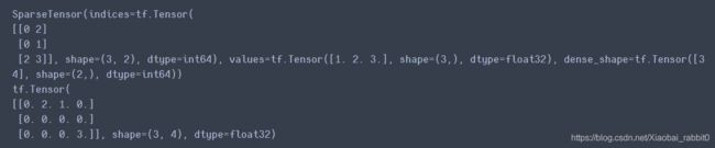
# sparse tensor
s5 = tf.SparseTensor(indices = [[0,2],[0,1],[2,3]],     #indices当顺序不正确的时候 调用to_dense（）时会报错
                    values = [1.,2.,3.],
                    dense_shape = [3,4])
print(s5)
s6 = tf.sparse.reorder(s5)      #排序
print(tf.sparse.to_dense(s6))

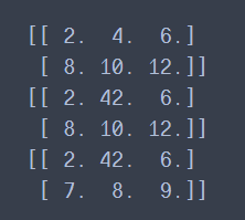
变量 Variables

# Variables
v = tf.Variable([[1.,2.,3.],[4.,5.,6.]])
print(v)
print(v.value())
print(v.numpy())

#变量重新赋值
v.assign(2*v)    #给变量重新赋值
print(v.numpy())
v[0,1].assign(42)    #具体位置赋值
print(v.numpy())
v[1].assign([7.,8.,9.])   #某一行赋值
print(v.numpy())

try:
    v[1] = [7.,8.,9.]
except TypeError as  ex:
    print(ex)

2 自定义损失函数与DenseLayer

2.1、自定义损失函数

• 构建模型

#自定义损失函数
def customized_mse(y_true,y_pred):
    mse = tf.reduce_mean(tf.square(y_pred - y_true))    #均方差
    return mse


#构建模型
model = keras.models.Sequential([
    keras.layers.Dense(30,activation='relu',input_shape=x_train.shape[1:]),   #这里取8(读取第二维的长度)，因为x_train.shape -> (11610,8)
    keras.layers.Dense(1),
])

model.summary()    #打印model的信息
model.compile(loss=customized_mse,optimizer="sgd",metrics=["mean_squared_error"])   #编译
callbacks = [keras.callbacks.EarlyStopping(patience = 5, min_delta = 1e-3)]

• 训练模型

#训练模型
history = model.fit(x_train_scaled, y_train, 
                    validation_data = (x_valid_scaled, y_valid), 
                    epochs = 100,
                    callbacks = callbacks)

由上述训练结果可以看出 自定义损失函数和mean_squared_error效果一样

2.2、自定义层次

DenseLayer

#customized dense layer   自定义全连接层
class CustomizedDenseLayer(keras.layers.Layer):
    def __init__(self,units,activation = None,**kwargs):    #初始化函数
        self.units = units              #这一层输出由几个单元
        self.activation = keras.layers.Activation(activation)
        super(CustomizedDenseLayer,self).__init__(**kwargs)     #调用父类函数
        
    def build(self,input_shape):   #负责参数初始化
        '''构建需要的参数'''
        #x * w + b    input_shape:[None,a]  w:[a,b]  output_shape:[None,b]
        self.kernel = self.add_weight(name = 'kernel',
                                      shape = (input_shape[1],self.units),
                                      initializer = 'uniform',    #使用均匀分布的方法去初始化kernel
                                      trainable = True)    #可训练
        self.bias = self.add_weight(name = 'bias',
                                    shape = (self.units,),
                                    initializer = 'zeros',
                                    trainable = True)
        super(CustomizedDenseLayer,self).build(input_shape)
        
    
    def call(self,x):              #完成一次正向计算
        '''需要完成正向计算'''
        return self.activation(x @ self.kernel + self.bias)

#构建模型
model = keras.models.Sequential([
#   keras.layers.Dense(30,activation='relu',input_shape=x_train.shape[1:]),   #这里取8(读取第二维的长度)，因为x_train.shape -> (11610,8)
#   keras.layers.Dense(1),
    CustomizedDenseLayer(30,activation='relu',input_shape=x_train.shape[1:]),   #这里取8(读取第二维的长度)，因为x_train.shape -> (11610,8)
    CustomizedDenseLayer(1),
])

model.summary()    #打印model的信息
model.compile(loss="mean_squared_error",optimizer="sgd")   #编译
callbacks = [keras.callbacks.EarlyStopping(patience = 5, min_delta = 1e-3)]

对于DenseLayer这种自带参数的层，我们定义了一个这样的子类。

如果是想把一个简单的函数定义为一个层次，没有参数build()函数也就不需要了，整个类比较小，这样写不雅观。所以，对于没有参数的函数，想把它们定义为层次的时候可以选择使用，lambda的方式自定义层次。

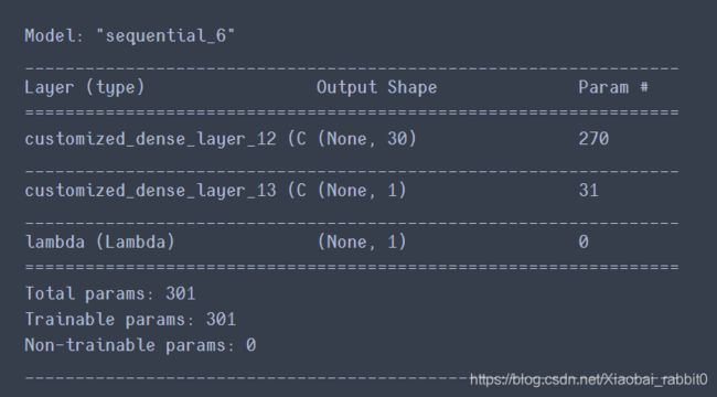
#lambda的方式自定义层次
'''eg:将激活函数定义为一个层  tf.nn.softplus : log(1 + e^x)'''
customized_softplus = keras.layers.Lambda(lambda x : tf.nn.softplus(x))
print(customized_softplus([-10.,-5.,0.,5.,10.]))

#customized dense layer   自定义全连接层
class CustomizedDenseLayer(keras.layers.Layer):
    def __init__(self,units,activation = None,**kwargs):    #初始化函数
        self.units = units              #这一层输出由几个单元
        self.activation = keras.layers.Activation(activation)
        super(CustomizedDenseLayer,self).__init__(**kwargs)     #调用父类函数
        
    def build(self,input_shape):   #负责参数初始化
        '''构建需要的参数'''
        #x * w + b    input_shape:[None,a]  w:[a,b]  output_shape:[None,b]
        self.kernel = self.add_weight(name = 'kernel',
                                      shape = (input_shape[1],self.units),
                                      initializer = 'uniform',    #使用均匀分布的方法去初始化kernel
                                      trainable = True)    #可训练
        self.bias = self.add_weight(name = 'bias',
                                    shape = (self.units,),
                                    initializer = 'zeros',
                                    trainable = True)
        super(CustomizedDenseLayer,self).build(input_shape)
        
    
    def call(self,x):              #完成一次正向计算
        '''需要完成正向计算'''
        return self.activation(x @ self.kernel + self.bias)

#构建模型
model = keras.models.Sequential([
#   keras.layers.Dense(30,activation='relu',input_shape=x_train.shape[1:]),   #这里取8(读取第二维的长度)，因为x_train.shape -> (11610,8)
#   keras.layers.Dense(1),
    CustomizedDenseLayer(30,activation='relu',input_shape=x_train.shape[1:]),   #这里取8(读取第二维的长度)，因为x_train.shape -> (11610,8)
    CustomizedDenseLayer(1),
    #加一个自定义的激活函数层
    customized_softplus,   #等价于下面两种代码
# '''
#     keras.layers.Dense(1,activation = "softplus")
#     #或
#     keras.layers.Dense(1),
#     keras.layers.Activation('softplus')
#     #或
# '''
    
])

model.summary()    #打印model的信息
model.compile(loss="mean_squared_error",optimizer="sgd")   #编译
callbacks = [keras.callbacks.EarlyStopping(patience = 5, min_delta = 1e-3)]

3 tf.function函数转换

import matplotlib as mpl
import matplotlib.pyplot as plt
%matplotlib inline
import numpy as np
import sklearn
import pandas as pd
import os
import sys
import time
import tensorflow as tf

from tensorflow import keras
#import keras

print(tf.__version__)
print(sys.version_info)
for module in mpl,np,pd,sklearn,tf,keras:
    print(module.__name__,module.__version__)

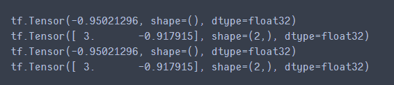
• tf.function函数转换python代码—1

#讲两个东西   1、tf.function   2、auto-graph
def scaled_elu(z,scale=1.0,alpha=1.0):
    # z >= 0 ? scale * z : scale * alpha * tf.nn.elu(z)
    is_positive = tf.greater_equal(z,0.0)     #判断z是否>0
    return scale * tf.where(is_positive,z,alpha * tf.nn.elu(z))   #三元表达式，tf中用where实现三元表达式

print(scaled_elu(tf.constant(-3.)))
print(scaled_elu(tf.constant([3.,-2.5])))

#一行代码，将python实现的函数转换成，tf中图实现的函数(tf图结构里面有很多优化，最大的优点就是：快！！！)
scaled_elu_tf = tf.function(scaled_elu)

print(scaled_elu_tf(tf.constant(-3.)))
print(scaled_elu_tf(tf.constant([3.,-2.5])))

#将python实现的函数转换成，tf中图实现的函数(tf图结构里面有很多优化，最大的优点就是：快！！！)
#下面做一个测试
%timeit scaled_elu(tf.random.normal((1000,1000)))
%timeit scaled_elu_tf(tf.random.normal((1000,1000)))

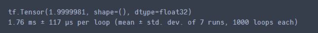
• tf.function函数转换python代码—2

'''举个例子'''
#1 + 1/2 + 1/2^2 + ... + 1/2^n

def converge_to_2(n_iters):
    total = tf.constant(0.)
    increment = tf.constant(1.)
    for _ in range(n_iters):
        total += increment
        increment /= 2.0
    return total

print(converge_to_2(20))
%timeit converge_to_2(20)

#加一个代码，也可以将代码转换为tf中的图
@tf.function

def converge_to_2(n_iters):
    total = tf.constant(0.)
    increment = tf.constant(1.)
    for _ in range(n_iters):
        total += increment
        increment /= 2.0
    return total

print(converge_to_2(20))
%timeit converge_to_2(20)

查看如何将python代码转换为tf图结构的

'''用auto-graph函数查看python代码如何转换为tf图结构的'''
def display_tf_code(func):
    code = tf.autograph.to_code(func)
    from IPython.display import display,Markdown
    display(Markdown('```python```'.format(code)))

display_tf_code(scaled_elu)

display_tf_code(converge_to_2)

注：使用@tf.function时 里面不能定义变量，需要放在外面，否则会报错

#  注：使用@tf.function时   里面不能定义变量，需要放在外面

var = tf.Variable(0.)      #变量的定义写在@tf.function函数外面

@tf.function
def add_21():
    return var.assign_add(21)  #  +=

print(add_21)

#添加input_signature限定类型

@tf.function(input_signature=[tf.TensorSpec([None],tf.int32,name='x')])

def cube(z):
    return tf.pow(z,3)
try:
    print(cube(tf.constant([1.,2.,3.])))
except ValueError as ex:
    print(ex)

print(cube(tf.constant([1,2,3])))

4 函数签名（类型）与图结构

这部分内容，与训练model没有关系。这些函数会用在两个地方：
1、如何保存模型；
2、保存好模型，要使用这个模型的时候，怎么载入模型
（get_operation_by_name，get_tensor_by_name）

5、自定义求导（近似求导）

5.1、python自定义，求导

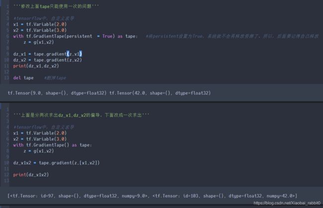
5.2、tf.GradientTape基本使用方法

• tf.GradientTape基本使用方法

'''tf.GradientTape基本使用方法'''
#tensorflow中，自定义求导
x1 = tf.Variable(2.0)
x2 = tf.Variable(3.0)
with tf.GradientTape() as tape:
    z = g(x1,x2)
    
dz_x1 = tape.gradient(z,x1)
print(dz_x1)

#tape 只能使用一次。因为，调用一次tape.gradient，tape就会自动被释放了，无法再用
#所以，这里先用try 抓住这个error
try:
    dz_x2 = tape.gradient(z,x2)
except RuntimeError as ex:
    print(ex)

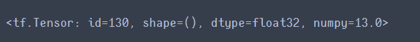
• 两个目标函数，对一个变量求导

'''两个目标函数，对一个变量求导'''
x = tf.Variable(5.0)
with tf.GradientTape() as tape:
    z1 = 3 * x
    z2 = x ** 2
tape.gradient([z1,z2],x)

• 求二阶导数，使用嵌套方法实现

'''求二阶导数，使用嵌套方法实现'''
#tensorflow中，自定义求导
x1 = tf.Variable(2.0)
x2 = tf.Variable(3.0)
with tf.GradientTape(persistent  = True) as outer_tape:  
    with tf.GradientTape(persistent  = True) as inner_tape:  
        z = g(x1,x2)
    inner_grads = inner_tape.gradient(z,[x1,x2])
outer_grads = [outer_tape.gradient(inner_grad,[x1,x2])
               for inner_grad in inner_grads]

print(outer_grads)

del inner_tape
del outer_tape
    

• 模拟梯度下降法

#模拟梯度下降法
learning_rate = 0.1
x = tf.Variable(0.0)

for _ in range(100):
    with tf.GradientTape() as tape:
        z = f(x)
    dz_dx = tape.gradient(z,x)
    x.assign_sub(learning_rate * dz_dx)
print(x)

• GradientTape与optimizer结合

#GradientTape与optimizer结合

learning_rate = 0.1
x = tf.Variable(0.0)

optimizer = keras.optimizers.SGD(lr = learning_rate)
for _ in range(100):
    with tf.GradientTape() as tape:
        z = f(x)
    dz_dx = tape.gradient(z,x)
    
    #x.assign_sub(learning_rate * dz_dx)
    optimizer.apply_gradients([(dz_dx,x)])
    
print(x)

5.3、tf.GradientTape与tf.keras结合使用

手动求导方式，对回归问题的求解

'''回归一下在fit函数中都做过什么'''
# 1.batch 遍历训练集  metric
    #1.1 自动求导
# 2.epoch结束  验证集 metric


#遍历训练集
epochs = 100    #遍历100次
batch_size = 32
steps_per_epoch = len(x_train_scaled) // batch_size    #训练多少次
optimizer = keras.optimizers.SGD()   #优化函数（这里lr使用默认值）
metric = keras.metrics.MeanSquaredError()    #均方差损失

#数据如何遍历
def random_batch(x,y,batch_size=32):
    idx = np.random.randint(0,len(x),size=batch_size)  #随机出32个索引
    return x[idx],y[idx]           #这里因为是numpy数据 所以idx是个列表，这样y[idx] 对应的就是数据了

#构建模型
model = keras.models.Sequential([
    keras.layers.Dense(30,activation='relu',input_shape=x_train.shape[1:]),   #这里取8(读取第二维的长度)，因为x_train.shape -> (11610,8)
    keras.layers.Dense(1),
])

for epoch in range(epochs):
    metric.reset_states()
    for step in range(steps_per_epoch):
        x_batch,y_batch = random_batch(x_train_scaled,y_train,batch_size)    #取出数据
        with tf.GradientTape() as tape:    
            y_pred = model(x_batch)      #获取预测值
            loss = tf.reduce_mean(keras.losses.mean_squared_error(y_batch,y_pred))   #有预测值之后，计算损失（均方误差）
            metric(y_batch,y_pred)     #累计计算metric
        grads = tape.gradient(loss,model.variables)    #求梯度
        grads_and_vars = zip(grads,model.variables)    #梯度和变量绑定
        optimizer.apply_gradients(grads_and_vars)      #梯度更新
        print("\rEpoch",epoch,"train mse:",metric.result().numpy(),end="")   #打印出来
    y_valid_pred = model(x_valid_scaled)     #验证集验证
    valid_loss = tf.reduce_mean(keras.losses.mean_squared_error(y_valid_pred,y_valid))
    print("\t","valid mse:",valid_loss.numpy())

其中，后面的for循环替代了之前用到的fit函数

6、章节总结

• 基础API
• 基础API与keras的集成
  • 自定义损失函数
  • 自定义层次
• @tf.function的使用
  • 图结构
• 自定义求导