反向传播算法的直观理解
定义 (DEFINITIONS)
DEFINITION 1. FORWARD PROPAGATION
定义1.向前传播
Normally, when we use a neural network we input some vector x and the network produces an out put y. The input vector goes through each hidden layer, one by one, until the output layer. Flow in this direction, is called forward propagation.
通常,当我们使用神经网络时,我们输入一些向量x,并且网络会产生输出y。 输入向量逐个遍历每个隐藏层,直到输出层。 沿这个方向的流动称为正向传播。
During the training stage, the input gets carried forward and at the end produces an scalar cost J(θ).
在训练阶段,输入被结转,最后产生标量成本J(θ)。
DEFINITION 2. BACK PROPAGATION ALGORITHM
定义2.反向传播算法
The back-prop algorithm then goes back into the network and adjusts the weights to compute the gradient. To be continued…
反向传播算法然后返回网络并调整权重以计算梯度。 未完待续…
DEFINITION 3. ANALYTICAL DIFFERENTIATION
定义3.分析鉴别
Doing it analytically in terms of algebra is probably what you did in school. For common functions, this is straightforward. But when an analytical method fails or is difficult, we usually try numerical differentiation.
从代数角度进行分析可能是您在学校所做的。 对于常见功能,这很简单。 但是当分析方法失败或困难时,我们通常会尝试数值微分。
DEFINITION 4. NUMERICAL DIFFERENTIATION
定义4.数值微分
Since algebraic manipulation is difficult or not possible, with numerical methods we general use methods that are heavy in calculation, therefore computers are often used. Numerical differentiation is done using discrete points of a function. From here there are 2 general methods: one is using the nearby points, while the other is using curve fitting.
由于很难或不可能进行代数运算,因此对于数值方法,我们通常使用计算量大的方法,因此经常使用计算机。 使用函数的离散点进行数值微分。 从这里开始,有2种常规方法:一种是使用附近的点,另一种是使用曲线拟合。
DEFINITION 5. STOCHASTIC GRADIENT DESCENT
定义5.随机梯度下降
The algorithm responsible for the “learning”. It uses the gradient produced by the back propagation algorithm.
负责“学习”的算法。 它使用反向传播算法产生的梯度。
DEFINITION 6. BACK PROPAGATION ALGORITHM
定义6.反向传播算法
The back-prop algorithm then goes back into the network and adjusts the weights to compute the gradient. In general, the back-prop algorithm is not just for multi-layer perceptron(s). Its a generic numerical differentiation algorithm that can be used to find the derivative of any function, given that the function is differentiable in the first place.
反向传播算法然后返回网络并调整权重以计算梯度。 通常,反向传播算法不仅适用于多层感知器。 它是一种通用的数值微分算法,可用于查找任何函数的导数,前提是该函数首先是可微的。
One of the top features of this algorithm is that it uses a relatively simple and inexpensive procedure to compute the differential. Making it quite efficient.
该算法的主要特点之一是它使用相对简单且便宜的过程来计算差分。 使其效率很高。
PROBLEM 1. HOW TO COMPUTE THE GRADIENT OF A COST FUNCTION
问题1.如何计算成本函数的梯度
Given a function f, we wanna find the gradient:
给定一个函数f,我们想找到梯度:
where x is a set of variables whose derivatives we need, and y are additional variables, that we don’t require the derivatives.
其中x是我们需要其导数的一组变量,而y是我们不需要导数的其他变量。
For learning, we want to find the gradient of the cost function. To be continued…
为了学习,我们想找到成本函数的梯度。 未完待续…
DEFINITION 6. LOSS FUNCTION
定义6.损失功能
This is the function applied to often one data point to find the delta between the predicted point and the actual point for example. Most times this is the squared loss, which gives the distance measure.
此函数通常应用于一个数据点,以查找例如预测点和实际点之间的增量。 大多数情况下,这是平方损失,它给出了距离度量。
DEFINITION 7. COST FUNCTION
定义7.成本函数
This is the function that is the combination of all the loss functions, it’s not always a sum. But sometimes an average or weighted average. For example:
该函数是所有损失函数的组合,并不总是求和。 但有时是平均值或加权平均值。 例如:
PROBLEM 1. HOW TO COMPUTE THE GRADIENT OF A COST FUNCTION
问题1.如何计算成本函数的梯度
Given a function f, we wanna find the gradient:
给定一个函数f,我们想找到梯度:
where x is a set of variables whose derivatives we need, and y are additional variables, that we don’t require the derivatives.
其中x是我们需要其导数的一组变量,而y是我们不需要导数的其他变量。
For learning, we want to find the gradient of the cost function.
为了学习,我们想找到成本函数的梯度。
To be continued…
未完待续…
DEFINITION 8. CHAIN RULE OF CALCULUS
定义8.算子的链规则
Given that x is a real number, and f and g are both functions mapping from a real number to real number. Furthermore,
假设x是一个实数,并且f和g都是从实数到实数的映射函数。 此外,
Then the chain rule says that,
然后链条规则说,
DEFINITION 9. MULTI-VARIABLE CHAIN RULE
定义9.多元链规则
Given that x and y are vectors in different dimensions,
假设x和y是不同维度的向量,
Also g and f are functions mapping from one dimension to another, such that,
g和f也是从一个维度映射到另一维度的函数,这样,
or equivalently,
或等效地,
where, ∂ y / ∂ x is the n × m Jacobian matrix of g.
,y /∂x是g的n×m雅可比矩阵。
DEFINITION 10. GRADIENT Whereas a derivative or differential is the rate of change along one axis. The gradient is a vector of slopes for a function along multiple axes.
定义10.梯度导数或微分是沿一个轴的变化率。 梯度是函数沿多个轴的斜率矢量。
DEFINITION 11. JACOBIAN MATRIX
定义11.雅各宾矩阵
Sometimes we need to find all of the partial derivatives of a function whose input and output are both vectors. The matrix containing all such partial derivatives is the Jacobian.
有时我们需要找到一个函数的所有偏导数,这些函数的输入和输出都是矢量。 包含所有此类偏导数的矩阵为雅可比行列式。
Given:
鉴于:
The Jacobian matrix J is given by:
雅可比矩阵J由下式给出:
DEFINITION 12. CHAIN RULE FOR TENSORS
定义12.张量链规则
We work with very high dimensional data most times, for example images and videos. So we need to extend our chain rule to beyond just vectors, into tensors.
大多数时候,我们使用非常高维度的数据,例如图像和视频。 因此,我们需要将链式规则扩展到不仅仅是矢量,还可以是张量。
Imagine a 3D tensor,
想象一下3D张量
The gradient of a value z with respect to this tensor is,
值z相对于该张量的梯度为,
For this tensor, the iᵗʰ index gives a tuple of 3 values, or a vector,
对于该张量,iᵗʰ索引给出一个包含3个值或向量的元组,
The gradient of a value z with respect to the iᵗʰ index of the tensor is,
值z相对于张量的iᵗʰ索引的梯度为
So given this,
因此,鉴于此,
The chain rule for tensors is,
张量的链式规则是
概念 (CONCEPTS)
CONCEPT 1. THE COMPUTATIONAL GRAPH
概念1.计算图
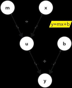
This is an example of a computational graph for the equation of a line. Starting nodes are what you will see in the equation, for the sake of the diagram, there’s always a need to define additional variables for intermediate nodes, in this example the node “u”. The node “u” is equivalent to “mx”.
这是直线方程的计算图示例。 起始节点是您将在方程式中看到的,为了方便起见,始终需要为中间节点定义其他变量,在本示例中为节点“ u”。 节点“ u”等效于“ mx”。
We introduce this concept to illustrate the complicated flow of computations in the back-prop algorithm.
我们引入这个概念来说明反向传播算法中复杂的计算流程。
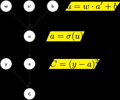
Remember from earlier, when we defined loss function to be a difference squared, that’s what we use here on the last layer of the computation graph. Where y is the actual value and a is the predicted value.
记得从前,当我们将损失函数定义为差平方时,这就是我们在计算图的最后一层使用的方法。 其中,y是实际值,a是预测值。
CONCEPT 2. FORWARD & BACKWARD PROPAGATION
概念2。向前和向后传播
Notice that our loss value is heavily dependent on the last activation value, which is then dependent on the previous activation value, which is then dependent on the preceding activation value and so on.
请注意,我们的损失值在很大程度上取决于上一个激活值,然后又取决于之前的激活值,然后又取决于之前的激活值,依此类推。
In going forward through the neural net, we end up with a predicted value, a. During the training stage, we have an additional information which is the actual result the network should get, y. Our loss function is really the distance between these value. When we wanna minimize this distance, we first have to update the weights on the very last layer. But this last layer is dependent on it’s preceding layer, therefore we update those. So in this sense we are propagating backwards through the neural network and updating each layer.
在遍历神经网络时,我们得出的预测值为a。 在培训阶段,我们还有其他信息,即网络应获得的实际结果y。 我们的损失函数实际上就是这些值之间的距离。 当我们想最小化此距离时,我们首先必须更新最后一层的权重。 但是最后一层取决于它的上一层,因此我们对它们进行更新。 因此,从这个意义上讲,我们正在通过神经网络向后传播并更新每一层。
CONCEPT 3. SENSITIVITY TO CHANGE
概念3.改变的敏感性
When a small change in x produces a large change in the function f, we say the the function is very sensitive to x. And if a small change in x produces a small change in f, we say it’s not very sensitive.
当x的较小变化导致函数f的较大变化时,我们说该函数对x非常敏感。 而且,如果x的微小变化导致f的微小变化,我们说它不是很敏感。
For example, the effectiveness of a drug may be measured by f, and x is the dosage used. The sensitivity is denoted by:
例如,药物的有效性可以通过f来测量,并且x是所使用的剂量。 灵敏度表示为:
To extend this further, let’s say our function was multi-variable now.
为了进一步扩展这一点,假设我们的函数现在是多变量的。
The function f can have different sensitivities to each input. So for example, maybe just quantity analysis wasn’t enough, so we break down the drug into 3 active ingredients and consider each one’s dosage.
函数f对每个输入可能具有不同的灵敏度。 因此,例如,也许仅仅进行数量分析还不够,因此我们将药物分为3种有效成分,并考虑每个人的剂量。
And the last bit of extension, if one of the input values, for example x is also dependent on it’s own inputs. We can use the chain rule to find those sensitivities. Again with the same example, maybe the x is broken down into it’s constituent parts in the body, so we have to consider that as well.
还有扩展的最后一位,如果输入值之一(例如x)也取决于它自己的输入。 我们可以使用链式规则找到那些敏感度。 再次使用相同的示例,也许x被分解为它在人体中的组成部分,所以我们也必须考虑这一点。
We consider the make up of x, and how its ingredients may be affecting the overall effectiveness of the drug.
我们考虑x的组成,以及其成分可能如何影响药物的整体功效。
Here, we’re measuring the how sensitive the effect of the overall drug is to this small ingredient of the drug.
在这里,我们正在测量整个药物的效果对药物的这种小成分的敏感程度。
CONCEPT 4. A SIMPLISTIC MODEL
概念4.简单模型
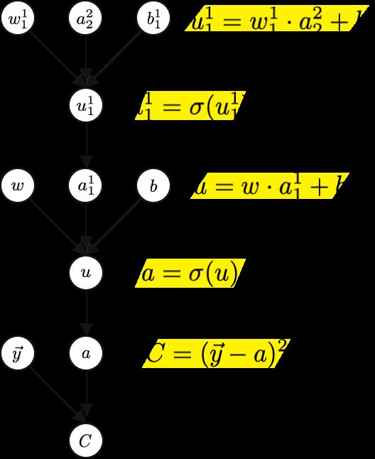
So this computation graph considers the link between the nodes a and the one right before it, a’.
因此,此计算图考虑了节点a和节点a'之间的链接。
To apply chain rule on this,
要对此应用连锁规则,
Which describes how sensitive C is to small changes in a. Then we move on to the preceding computation,
其中描述了C对a中的微小变化有多敏感。 然后我们继续前面的计算,
Which measures how sensitive a is to small changes in u. Then we move on to the preceding 3 computations,
哪个度量a对u的微小变化有多敏感。 然后我们继续前面的3个计算,
Which measures how sensitive u is to small changes in each of the:
哪个度量u对以下各项中的微小变化有多敏感:
- weight, w 重量,w
- preceding activation value, a’ 前一个激活值,a'
- bias, b 偏差,b
Putting this all together we get,
将所有这些放在一起,
CONCEPT 5. COMPLICATIONS WITH A SIMPLISTIC MODEL
概念5.简单模型的复杂化
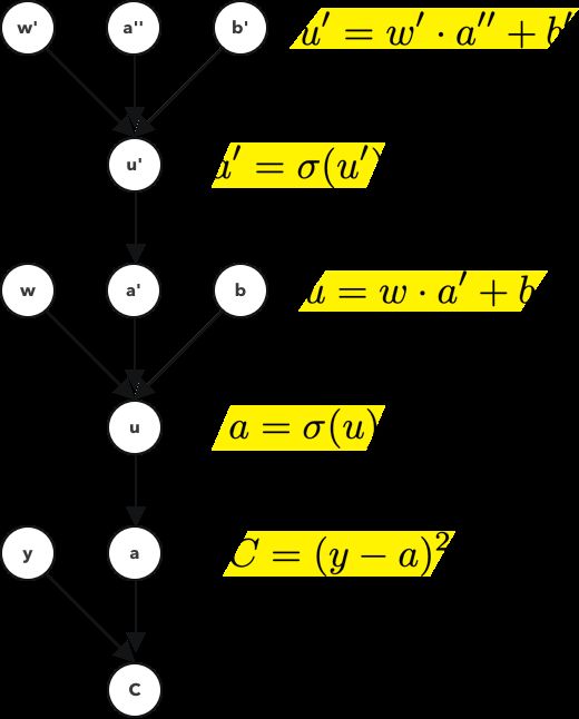
If in the previous example, we have 2 nodes and 1 link between them. With this example we have 3 nodes and 2 links.
如果在前面的示例中,我们有2个节点和它们之间的1个链接。 在此示例中,我们有3个节点和2个链接。
Since there’s no limit on how long you can chain the chain rule. We can keep doing this for arbitrary number of layers. For this layer, note that the computation graph becomes this,
由于对链接规则的链接时间没有限制。 我们可以继续对任意数量的层执行此操作。 对于这一层,请注意计算图变为
Notice the need to annotate each node with additional ticks. These ticks are not derivatives though, they just signify that u and u’ are different, unique values or objects.
注意,需要用附加的刻度标记每个节点。 尽管这些刻度不是派生的,它们只是表示u和u'是不同的,唯一的值或对象。
CONCEPT 5. COMPLICATIONS WITH A COMPLEX MODEL
概念5.复杂模型的复杂化
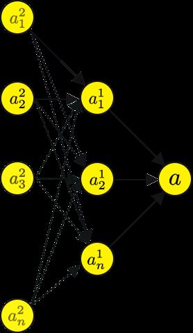
The examples so far have been linear, linked list kind of neural nets. To expand it to realistic networks, like this,
到目前为止,示例都是线性的,链表式的神经网络。 要将其扩展到现实的网络中,
We have to add some additional notation to our network.
我们必须在网络中添加一些其他符号。
Let’s see how we would get the computational graph for a²₁ through a¹₁.
让我们看看如何获得a²₁到a¹₁的计算图。
Now let’s see how we would get the computational graph for a²₂ through a¹₁.
现在,让我们看看如何得到a²2到a¹₁的计算图。
You will notice that both graphs actually have a large component in common, specifically everything up to a¹₁. Meaning that if a computation has already been computed, then it could be reused the next and the next time and so on. While this increases the use of memory, it significantly reduces compute time, and for a large neural net, is necessary.
您会注意到,两个图实际上有一个大的共同点,尤其是所有不超过a₁的东西。 这意味着,如果已经计算出一个计算,则可以在下一次和下一次重用它,依此类推。 尽管这增加了内存的使用量,但它显着减少了计算时间,并且对于大型神经网络而言,这是必需的。
If we use the chain rule on these, we get pretty much the same formulas, just with the additional indexing.
如果我们在这些规则上使用链式规则,我们将获得几乎相同的公式,只是带有附加索引。
CONCEPT 6. FURTHER COMPLICATIONS WITH A COMPLEX MODEL
概念6.复杂模型的进一步复杂化
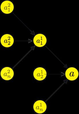
You will notice that a²₂ will actually have several paths back to the output layer node, like so.
您会注意到,a²²实际上将有几条返回输出层节点的路径,就像这样。
So this necessitates us to sum over the previous layer. This value that we get from the summation of all preceding nodes and their gradients has the instruction for updating it so that we minimize the error.
因此,这需要我们对上一层进行汇总。 我们从前面所有节点及其梯度的总和中获得的值具有更新该指令的指示,以便使误差最小化。
CONCEPT 7. MINIMIZING THE COST FUNCTION
概念7.最小化成本功能
If you remember DEFINITIONS 6 & 7, specifically 7, you’ll remember that the cost function is conceptually the average or the weighted average of the differences between the predicted and actual outputs.
如果您记得定义6和7,特别是7,则将记住成本函数在概念上是预测产出与实际产出之间差异的平均值或加权平均值。
If we use the Gradient Descent algorithm for Linear Regression or Logistic Regression to minimize the cost function.
如果我们使用线性线性回归或逻辑回归的梯度下降算法来最小化成本函数。
Then for Neural Networks we use the Back Propagation algorithm. I think by now it is clear why we can’t just use single equation for a neural network. Neural networks aren’t exactly continuous functions that we can find a nice derivative of. Rather they are discrete nodes that approximate a function in concert. Hence the need for a recursive algorithm to find it’s derivative or gradient, which takes into factor all the nodes.
然后对于神经网络,我们使用反向传播算法。 我认为到现在为止很清楚为什么我们不能只对神经网络使用单个方程式了。 神经网络并非完全连续的函数,我们可以找到它的一个很好的派生类。 相反,它们是离散的节点,它们近似地协调一个函数。 因此,需要一种递归算法来找到它的导数或梯度,这需要考虑所有节点。
The complete cost function looks something like this:
完整的成本函数如下所示:
Which is conceptually just:
从概念上讲,这仅仅是:
CONCEPT 7. SYMBOL TO SYMBOL DERIVATIVES
概念7.从符号到符号导数
So far you have an idea of how to get the algebraic expression for the gradient of a node in a neural network. Via the application of the chain rule to tensors and the concept of the computational graph.
到目前为止,您已经了解了如何获取神经网络中节点的梯度的代数表达式。 通过将链式规则应用于张量和计算图的概念。
The algebraic expression or the computational graph don’t deal with numbers, rather they just give us the theoretical background to verify that we are computing them correctly. And they help guide our coding.
代数表达式或计算图不处理数字,而是给我们提供理论背景以验证我们是否正确计算了它们。 它们有助于指导我们的编码。
In the next concept, we will talk about the symbol to number derivatives.
在下一个概念中,我们将讨论符号到数字的导数。
CONCEPT 8. SYMBOL TO NUMBER DERIVATIVES
概念8.符号到数字的导数
Here we start to depart from theory and go into the practical arena.
在这里,我们开始背离理论,进入实践领域。
算法 (ALGORITHMS)
ALGORITHM 1. BASIC SETUP + GET GRADIENT OF NODE
算法1.基本设置+结点梯度
First of all we have to make a few setups, first of those being, the order of the neural network and the computational graph of the nodes associated with our network. We order them in such a way that we the computation of one comes after the other.
首先,我们必须进行一些设置,首先是神经网络的顺序和与我们的网络关联的节点的计算图。 我们以这样一种方式对它们进行排序,使得我们一个计算在另一个计算之后。
Each node u^{(n)} is associated with an operation f^{(i)} such that:
每个节点u ^ {(n)}与操作f ^ {(i)}关联,这样:
where ^{(i)} is the set of all nodes that are the parent of u^{(n)}.
其中^ {(i)}是u ^ {(n)}父级的所有节点的集合。
First we need to compute get all the input nodes, to do that we need to input all the training data in the form of x vectors:
首先,我们需要计算获取所有输入节点,为此,我们需要以x向量的形式输入所有训练数据:
for i = 1, ...., n_i
	u_i = get_u(x_i)
Note that n_i is the number of input nodes, where the input nodes are:
请注意, n_i是输入节点的数量,其中输入节点为:
If these are input nodes, then the nodes:
如果这些是输入节点,那么这些节点:
are the nodes after the input nodes but before the last node, u^{(n)}.
是输入节点之后但最后一个节点u ^ {(n)}之前的节点。
for i = n_i+1, ..., n
	A_i = { u_j = get_j(Pa(u_i)) }
	u_i = fi(A_i)
You will notice that these go in the other direction than when we were conceptualizing the chain rule computational graph. This is because this algorithm details out the forward propagation.
您会注意到,这些方向与我们概念化链式规则计算图时的方向相反。 这是因为该算法详细说明了前向传播。
We will call this graph:
我们称这个图为:
Using this graph, we can construct another graph:
使用此图,我们可以构造另一个图:
While each node of G computes the forward graph node u^i, each node in B computes the gradients using the chain rule.
G的每个节点都计算前向图节点u ^ i时,B的每个节点都使用链规则计算梯度。
If you consider all the nodes in a neural network and the edges that connect them, you can think of the computation required to do back propagation increasing linearly with the number of edges. Since each edge represents the computation of one chain rule, connecting some node to one of its parent nodes.
如果考虑神经网络中的所有节点以及连接它们的边,则可以想到进行反向传播所需的计算量随边的数量线性增加。 由于每个边代表一个链规则的计算,因此将某个节点连接到其父节点之一。
ALGORITHM 2. ADDITIONAL CONSTRAINTS + SIMPLE BACK PROPAGATION
算法2.附加约束+简单的反向传播
As mentioned above, the computational complexity of the algorithm is linear with the number of edges of the network. But this is assuming that finding the partials on each edge is a constant time.
如上所述,算法的计算复杂度与网络边缘的数量成线性关系。 但这是假设在每个边缘上找到局部片段的时间是恒定的。
Here we aim to build a concrete understanding of the backprop algorithm while still keeping certain complications out of sight. One of them being the tensor nodes.
在这里,我们旨在建立对反向传播算法的具体理解,同时仍使某些复杂性看不见。 其中之一是张量节点。
Run forward propagationThis will obtain the activation values for the network, that are in randomized or not as useful state.
这将获得网络的激活值,这些激活值处于随机状态或不可用状态。
Initialize grad_tableIn this data structure we will store all the gradients that we compute.
在此数据结构中,我们将存储我们计算出的所有梯度。
To get an individual entry, we use grad_table(u_i)This will store the calculated value of:
这将存储以下内容的计算值:
grad_table[u_n] = 1This sets the last node to 1.
这会将最后一个节点设置为1。
for j = n-1 to 1
	grad_table[u_j] = \\sum grad_table[u_i] du_i/du_j
This is theoretically this:
理论上是这样的:
return grad_tableThe backprop algorithm visits each node only once to calculate the partials, this prevents the unnecessary recalculation of exponential number of sub expressions. Remember that this comes at the cost of more memory usage.
反向传播算法仅访问每个节点一次以计算局部变量,从而避免了不必要的子表达式指数数量的重新计算。 请记住,这是以更多的内存使用为代价的。
其他文章 (Other Articles)
This post is part of a series of stories that explores the fundamentals of deep learning:1. Linear Algebra Data Structures and OperationsObjects and Operations2. Computationally Efficient Matrices and Matrix Decompositions
Inverses, Linear Dependence, Eigen-decompositions, SVD3. Probability Theory Ideas and ConceptsDefinitions, Expectation, Variance4. Useful Probability Distributions and Structured Probabilistic ModelsActivation Functions, Measure and Information Theory5. Numerical Method Considerations for Machine Learning
Overflow, Underflow, Gradients and Gradient Based Optimizations6. Gradient Based Optimizations
Taylor Series, Constrained Optimization, Linear Least Squares7. Machine Learning Background Necessary for Deep Learning I
Generalization, MLE, Kullback-Leibler Divergence8. Machine Learning Background Necessary for Deep Learning II
Regularization, Capacity, Parameters, Hyper-parameters9. Principal Component Analysis Breakdown
Motivation, Derivation10. Feed-forward Neural Networks
Layers, definitions, Kernel Trick11. Gradient Based Optimizations Under The Deep Learning Lens
Stochastic Gradient Descent, Cost Function, Maximum Likelihood12. Output Units For Deep Learning
Stochastic Gradient Descent, Cost Function, Maximum Likelihood13. Hidden Units For Deep Learning
Activation Functions, Performance, Architecture14. The Common Approach to Binary ClassificationThe most generic way to setup your deep learning models to categorize movie reviews15. General Architectural Design Considerations for Neural NetworksUniversal Approximation Theorem, Depth, Connections16. Classifying Text Data into Multiple ClassesSingle-Label Multi-class Classification17. Back Propagation Algorithm Part IDefinitions, Concepts, Algorithms with Visuals
下一个… (Up Next…)
Coming up next is the Part II of this article. If you would like me to write another article explaining a topic in-depth, please leave a comment.
接下来是本文的第二部分 。 如果您希望我写另一篇文章深入解释某个主题,请发表评论。
For the table of contents and more content click here.
有关目录和更多内容,请单击此处 。
翻译自: https://medium.com/swlh/back-propagation-algorithm-85c65e6fc359
反向传播算法的直观理解


