机器学习手写多层神经网络实现猫的识别
本文基于吴恩达老师深度学习作业,用多层神经网络实现猫的识别。
-
-
- 准备第三方库
- 加载数据
- 查看数据
- 测试结果
- 先定义前向传播中的线性部分
- 线性激活部分
- 用交叉熵损失函数计算代价
- 定义sigmoid和Relu激活函数反向传播部分
- 完整反向传播函数
- 反向传播模型
- 更新参数
- 多层神经网络模型
- 开始训练
- 训练结果
- 用训练好的参数预测自己的图片
-
我们来说一下步骤:
初始化网络参数
前向传播
1 计算一层的中线性求和的部分
2计算激活函数的部分(ReLU使用L-1次,Sigmod使用1次)
3 结合线性求和与激活函数
计算误差
反向传播
1 线性部分的反向传播公式
2 激活函数部分的反向传播公式
3 结合线性部分与激活函数的反向传播公式
更新参数
准备第三方库
# 导入必要库
import numpy as np
import h5py
import scipy
from scipy import ndimage
import matplotlib.pyplot as plt
import testCases
from dnn_utils import sigmoid, sigmoid_backward, relu, relu_backward #参见资料包
import lr_utils
加载数据
数据来自吴恩达深度学习周四课程中的猫的图片数据
# 加载数据
train_set_x_orig , train_set_y , test_set_x_orig , test_set_y , classes = lr_utils.load_dataset()

train_x_flatten = train_set_x_orig.reshape(train_set_x_orig.shape[0], -1).T
test_x_flatten = test_set_x_orig.reshape(test_set_x_orig.shape[0], -1).T

train_x = train_x_flatten / 255
train_y = train_set_y
test_x = test_x_flatten / 255
test_y = test_set_y
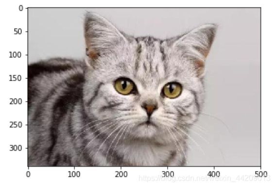
查看数据
index = 25
plt.imshow(train_set_x_orig[25]) #查看第26张图片
print(train_set_y) # 查看所有标签,1 猫    0 不是猫
[[0 0 1 0 0 0 0 1 0 0 0 1 0 1 1 0 0 0 0 1 0 0 0 0 1 1 0 1 0 1 0 0 0 0 0 0
  0 0 1 0 0 1 1 0 0 0 0 1 0 0 1 0 0 0 1 0 1 1 0 1 1 1 0 0 0 0 0 0 1 0 0 1
  0 0 0 0 0 0 0 0 0 0 0 1 1 0 0 0 1 0 0 0 1 1 1 0 0 1 0 0 0 0 1 0 1 0 1 1
  1 1 1 1 0 0 0 0 0 1 0 0 0 1 0 0 1 0 1 0 1 1 0 0 0 1 1 1 1 1 0 0 0 0 1 0
  1 1 1 0 1 1 0 0 0 1 0 0 1 0 0 0 0 0 1 0 1 0 1 0 0 1 1 1 0 0 1 1 0 1 0 1
  0 0 0 0 0 1 0 0 1 0 0 0 1 0 0 0 0 1 0 0 1 0 0 0 0 0 0 0 0]]
# 初始化神经网络结构
def initialize_parameters_deep(layers_dims):
    """
    此函数是为了初始化多层网络参数而使用的函数。
    参数:
        layers_dims - 包含我们网络中每个图层的节点数量的列表

    返回:
        parameters - 包含参数“W1”,“b1”,...,“WL”,“bL”的字典:
                     W1 - 权重矩阵,维度为(layers_dims [1],layers_dims [1-1])
                     bl - 偏向量,维度为(layers_dims [1],1)
    """
    np.random.seed(3)
    parameters = {}
    L = len(layers_dims)

    for l in range(1,L):
        parameters["W" + str(l)] = np.random.randn(layers_dims[l], layers_dims[l - 1]) / np.sqrt(layers_dims[l - 1])
        parameters["b" + str(l)] = np.zeros((layers_dims[l], 1))

        #确保我要的数据的格式是正确的
        assert(parameters["W" + str(l)].shape == (layers_dims[l], layers_dims[l-1]))
        assert(parameters["b" + str(l)].shape == (layers_dims[l], 1))

    return parameters
# 测试
initialize_parameters_deep(layers_dims = [5,4,4,1])
测试结果
{'W1': array([[ 0.79989897,  0.19521314,  0.04315498, -0.83337927, -0.12405178],
        [-0.15865304, -0.03700312, -0.28040323, -0.01959608, -0.21341839],
        [-0.58757818,  0.39561516,  0.39413741,  0.76454432,  0.02237573],
        [-0.18097724, -0.24389238, -0.69160568,  0.43932807, -0.49241241]]),
 'W2': array([[-0.59252326, -0.10282495,  0.74307418,  0.11835813],
        [-0.51189257, -0.3564966 ,  0.31262248, -0.08025668],
        [-0.38441818, -0.11501536,  0.37252813,  0.98805539],
        [-0.62206166, -0.31320846, -0.40188305, -1.20954159]]),
 'W3': array([[-0.46189601, -0.51193788,  0.56198898, -0.06595712]]),
 'b1': array([[0.],
        [0.],
        [0.],
        [0.]]),
 'b2': array([[0.],
        [0.],
        [0.],
        [0.]]),
 'b3': array([[0.]])}
先定义前向传播中的线性部分
# 前向传播线性部分
def linear_forward(A,W,b):
    """
    实现前向传播的线性部分。

    参数:
        A - 来自上一层(或输入数据)的激活,维度为(上一层的节点数量,示例的数量)
        W - 权重矩阵,numpy数组,维度为(当前图层的节点数量,前一图层的节点数量)
        b - 偏向量,numpy向量,维度为(当前图层节点数量,1)

    返回:
         Z - 激活功能的输入,也称为预激活参数
         cache - 一个包含“A”,“W”和“b”的字典,存储这些变量以有效地计算后向传递
    """
    Z = np.dot(W,A) + b
    assert(Z.shape == (W.shape[0],A.shape[1]))
    cache = (A,W,b)

    return Z,cache
线性激活部分
def linear_activation_forward(A_prev,W,b,activation):
    """
    实现LINEAR-> ACTIVATION 这一层的前向传播

    参数:
        A_prev - 来自上一层(或输入层)的激活,维度为(上一层的节点数量,示例数)
        W - 权重矩阵,numpy数组,维度为(当前层的节点数量,前一层的大小)
        b - 偏向量,numpy阵列,维度为(当前层的节点数量,1)
        activation - 选择在此层中使用的激活函数名,字符串类型,【"sigmoid" | "relu"】

    返回:
        A - 激活函数的输出,也称为激活后的值
        cache - 一个包含“linear_cache”和“activation_cache”的字典,我们需要存储它以有效地计算后向传递
    """

    if activation == "sigmoid":
        Z, linear_cache = linear_forward(A_prev, W, b)
        A, activation_cache = sigmoid(Z)  # return A & Z
    elif activation == "relu":
        Z, linear_cache = linear_forward(A_prev, W, b)
        A, activation_cache = relu(Z)

    assert(A.shape == (W.shape[0],A_prev.shape[1]))
    cache = (linear_cache,activation_cache)

    return A,cache
# 完整前向传播模型
def L_model_forward(X,parameters):
    """
    实现[LINEAR-> RELU] *(L-1) - > LINEAR-> SIGMOID计算前向传播,也就是多层网络的前向传播,为后面每一层都执行LINEAR和ACTIVATION

    参数:
        X - 数据,numpy数组,维度为(输入节点数量,示例数)
        parameters - initialize_parameters_deep()的输出

    返回:
        AL - 最后的激活值
        caches - 包含以下内容的缓存列表:
                 linear_relu_forward()的每个cache(有L-1个,索引为从0到L-2)
                 linear_sigmoid_forward()的cache(只有一个,索引为L-1)
    """
    caches = []
    A = X
    L = len(parameters) // 2

    # 前L-1层使用Relu激活函数,最后一层使用sigmoid激活函数
    for l in range(1,L):
        A_prev = A
        A, cache = linear_activation_forward(A_prev, parameters['W' + str(l)], parameters['b' + str(l)], "relu")
        caches.append(cache)

    AL,cache = linear_activation_forward(A, parameters['W'+str(L)], parameters['b'+str(L)], "sigmoid")
    caches.append(cache)

    return AL, caches
用交叉熵损失函数计算代价
# 计算成本
def compute_cost(AL,Y):
    """
    参数:
        AL - 与标签预测相对应的概率向量,维度为(1,示例数量)
        Y - 标签向量(例如:如果不是猫,则为0,如果是猫则为1),维度为(1,数量)

    返回:
        cost - 交叉熵成本
    """
    m = Y.shape[1]
    cost = -np.sum(np.multiply(np.log(AL),Y) + np.multiply(np.log(1 - AL), 1 - Y)) / m

    cost = np.squeeze(cost)
    assert(cost.shape == ())

    return cost
# 反向传播的线性部分
def linear_backward(dZ,cache):
    """
    为单层实现反向传播的线性部分(第L层)

    参数:
         dZ - 相对于(当前第l层的)线性输出的成本梯度
         cache - 来自当前层前向传播的值的元组(A_prev,W,b)

    返回:
         dA_prev - 相对于激活(前一层l-1)的成本梯度,与A_prev维度相同
         dW - 相对于W(当前层l)的成本梯度,与W的维度相同
         db - 相对于b(当前层l)的成本梯度,与b维度相同
    """
    A_prev, W, b = cache
    m = A_prev.shape[1]
    dW = np.dot(dZ, A_prev.T) / m
    db = np.sum(dZ, axis=1, keepdims=True) / m
    dA_prev = np.dot(W.T, dZ)

    assert (dA_prev.shape == A_prev.shape)
    assert (dW.shape == W.shape)
    assert (db.shape == b.shape)

    return dA_prev, dW, db
定义sigmoid和Relu激活函数反向传播部分
def sigmoid_backward(dA, cache):

    Z = cache
    s = 1/(1+np.exp(-Z))
    dZ = dA * s * (1-s)

    assert (dZ.shape == Z.shape)

    return dZ

def relu_backward(dA, cache):

    Z = cache
    dZ = np.array(dA, copy=True) # just converting dz to a correct object.

    dZ[Z <= 0] = 0

    assert (dZ.shape == Z.shape)

    return dZ
完整反向传播函数
def linear_activation_backward(dA,cache,activation="relu"):
    """
    实现LINEAR-> ACTIVATION层的后向传播。

    参数:
         dA - 当前层l的激活后的梯度值
         cache - 我们存储的用于有效计算反向传播的值的元组(值为linear_cache,activation_cache)
         activation - 要在此层中使用的激活函数名,字符串类型,【"sigmoid" | "relu"】
    返回:
         dA_prev - 相对于激活(前一层l-1)的成本梯度值,与A_prev维度相同
         dW - 相对于W(当前层l)的成本梯度值,与W的维度相同
         db - 相对于b(当前层l)的成本梯度值,与b的维度相同
    """
    linear_cache, activation_cache = cache
    if activation == "relu":
        dZ = relu_backward(dA, activation_cache)
        dA_prev, dW, db = linear_backward(dZ, linear_cache)
    elif activation == "sigmoid":
        dZ = sigmoid_backward(dA, activation_cache)
        dA_prev, dW, db = linear_backward(dZ, linear_cache)

    return dA_prev,dW,db
反向传播模型
def L_model_backward(AL,Y,caches):
    """
    对[LINEAR-> RELU] *(L-1) - > LINEAR - > SIGMOID组执行反向传播,就是多层网络的向后传播

    参数:
     AL - 概率向量,正向传播的输出(L_model_forward())
     Y - 标签向量(例如:如果不是猫,则为0,如果是猫则为1),维度为(1,数量)
     caches - 包含以下内容的cache列表:
                 linear_activation_forward("relu")的cache,不包含输出层
                 linear_activation_forward("sigmoid")的cache

    返回:
     grads - 具有梯度值的字典
              grads [“dA”+ str(l)] = ...
              grads [“dW”+ str(l)] = ...
              grads [“db”+ str(l)] = ...
    """
    grads = {}
    L = len(caches)
    m = AL.shape[1]
    Y = Y.reshape(AL.shape)
    dAL = - (np.divide(Y, AL) - np.divide(1 - Y, 1 - AL))

    current_cache = caches[L-1]
    grads["dA" + str(L)], grads["dW" + str(L)], grads["db" + str(L)] = linear_activation_backward(dAL, current_cache, "sigmoid")

    for l in reversed(range(L-1)):
        current_cache = caches[l]
        dA_prev_temp, dW_temp, db_temp = linear_activation_backward(grads["dA" + str(l + 2)], current_cache, "relu")
        grads["dA" + str(l + 1)] = dA_prev_temp
        grads["dW" + str(l + 1)] = dW_temp
        grads["db" + str(l + 1)] = db_temp

    return grads
更新参数
def update_parameters(parameters, grads, learning_rate):
    """
    使用梯度下降更新参数

    参数:
     parameters - 包含你的参数的字典
     grads - 包含梯度值的字典,是L_model_backward的输出

    返回:
     parameters - 包含更新参数的字典
                   参数[“W”+ str(l)] = ...
                   参数[“b”+ str(l)] = ...
    """
    L = len(parameters) // 2 #整除
    for l in range(L):
        parameters["W" + str(l + 1)] = parameters["W" + str(l + 1)] - learning_rate * grads["dW" + str(l + 1)]
        parameters["b" + str(l + 1)] = parameters["b" + str(l + 1)] - learning_rate * grads["db" + str(l + 1)]

    return parameters
多层神经网络模型
def L_layer_model(X, Y, layers_dims, learning_rate=0.0075, num_iterations=3000, print_cost=False,isPlot=True):
    """
    实现一个L层神经网络:[LINEAR-> RELU] *(L-1) - > LINEAR-> SIGMOID。

    参数:
        X - 输入的数据,维度为(n_x,例子数)
        Y - 标签,向量,0为非猫,1为猫,维度为(1,数量)
        layers_dims - 层数的向量,维度为(n_y,n_h,···,n_h,n_y)
        learning_rate - 学习率
        num_iterations - 迭代的次数
        print_cost - 是否打印成本值,每100次打印一次
        isPlot - 是否绘制出误差值的图谱

    返回:
     parameters - 模型学习的参数。 然后他们可以用来预测。
    """
    np.random.seed(1)
    costs = []

    parameters = initialize_parameters_deep(layers_dims)

    for i in range(0,num_iterations):
        AL , caches = L_model_forward(X,parameters)

        cost = compute_cost(AL,Y)

        grads = L_model_backward(AL,Y,caches)

        parameters = update_parameters(parameters,grads,learning_rate)

        #打印成本值,如果print_cost=False则忽略
        if i % 100 == 0:
            #记录成本
            costs.append(cost)
            #是否打印成本值
            if print_cost:
                print("第", i ,"次迭代,成本值为:" ,np.squeeze(cost))
    #迭代完成,根据条件绘制图
    if isPlot:
        plt.plot(np.squeeze(costs))
        plt.ylabel('cost')
        plt.xlabel('iterations (per tens)')
        plt.title("Learning rate =" + str(learning_rate))
        plt.show()
    return parameters
# 预测函数
def predict(X, y, parameters):
    """
    该函数用于预测L层神经网络的结果,当然也包含两层

    参数:
     X - 测试集
     y - 标签
     parameters - 训练模型的参数

    返回:
     p - 给定数据集X的预测
    """

    m = X.shape[1]
    n = len(parameters) // 2 # 神经网络的层数
    p = np.zeros((1,m))

    #根据参数前向传播
    probas, caches = L_model_forward(X, parameters)

    for i in range(0, probas.shape[1]):
        if probas[0,i] > 0.5:
            p[0,i] = 1
        else:
            p[0,i] = 0

    print("准确度为: "  + str(float(np.sum((p == y))/m)))

    return p
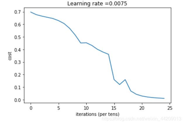
开始训练
layers_dims = [12288, 5, 5, 5, 1] # 神经网络结构
parameters = L_layer_model(train_x, train_y, layers_dims, num_iterations = 2500, print_cost = True,isPlot=True)
训练结果
第 0 次迭代,成本值为: 0.6978343828561023
第 100 次迭代,成本值为: 0.677132430616011
第 200 次迭代,成本值为: 0.6654901610560577
第 300 次迭代,成本值为: 0.6558182563579574
第 400 次迭代,成本值为: 0.6462338773043887
第 500 次迭代,成本值为: 0.629556239504452
第 600 次迭代,成本值为: 0.6064716676762193
第 700 次迭代,成本值为: 0.5682128757590694
第 800 次迭代,成本值为: 0.5150993982487242
第 900 次迭代,成本值为: 0.45119773439072314
第 1000 次迭代,成本值为: 0.45320425106544443
第 1100 次迭代,成本值为: 0.43195959636341597
第 1200 次迭代,成本值为: 0.4011698565079565
第 1300 次迭代,成本值为: 0.3792819244178975
第 1400 次迭代,成本值为: 0.3612456937302191
第 1500 次迭代,成本值为: 0.15978415024822354
第 1600 次迭代,成本值为: 0.12024692222669645
第 1700 次迭代,成本值为: 0.15938383021735222
第 1800 次迭代,成本值为: 0.06896835915402598
第 1900 次迭代,成本值为: 0.04264941082744414
第 2000 次迭代,成本值为: 0.029008712045154702
第 2100 次迭代,成本值为: 0.021005467409719286
第 2200 次迭代,成本值为: 0.015947431793655677
第 2300 次迭代,成本值为: 0.012568847909837035
第 2400 次迭代,成本值为: 0.010198826192851727
predictions_train = predict(train_x, train_y, parameters) #训练集
predictions_test = predict(test_x, test_y, parameters) #测试集
准确度为: 1.0
准确度为: 0.76
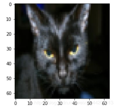
用训练好的参数预测自己的图片
my_image = "1.jpg"
my_label_y = [1]
## END CODE HERE ##

fname = "测试图片/" + my_image
image = np.array(scipy.ndimage.imread(fname, flatten=False))
my_image = scipy.misc.imresize(image, size=(64,64)).reshape((64*64*3,1))
my_predicted_image = predict(my_image, my_label_y, parameters)

plt.imshow(image)
print ("y = " + str(np.squeeze(my_predicted_image)) + ", your L-layer model predicts a \"" + classes[int(np.squeeze(my_predicted_image)),].decode("utf-8") +  "\" picture.")
准确度为: 1.0
y = 1.0, your L-layer model predicts a "cat" picture.