【强化学习】 Nature DQN算法与莫烦代码重现（tensorflow)

DQN,(Deep Q-Learning)是将深度学习与强化学习相结合。在Q-learning中，我们是根据不断更新Q-table中的值来进行训练。但是在数据量比较大的情况下，Q-table是无法容纳所有的数据量，因此提出了DQN。DQN的核心就是把Q-table的更新转化为函数问题，通过拟合一个function来代替Q-table产生Q值。

一、DQN算法原理

强化学习算法可以分为三大类：value based,policy based和actor critic。以DQN为代表的是value based算法，这种算法只有一个值函数网络，没有policy网络。

在DQN（NIPS 2013）里面，我们使用的目标Q值的计算方式为：

这里目标Q值的计算使用到了当前要训练的Q网络参数来计算，但实际上，我们又通过yj来更新Q网络参数。两者循环依赖，迭代起来相关性太强，不利于算法的收敛。因此一个改版的DQN：Nature DQN尝试使用两个网络结构完全相同的神经网络来减少目标Q值计算和要更新Q网络参数之间的依赖关系。下面是对Nature DQN的介绍（以下Nature DQN 均称DQN）。

二、Nature DQN结构简介

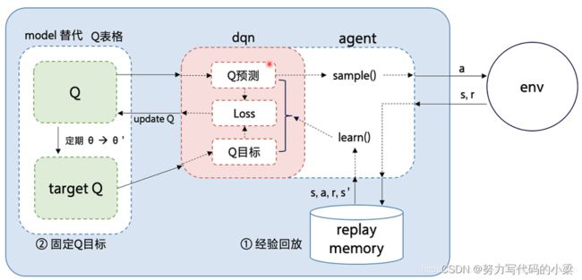
DQN和Qlearning一样，都是采用off-policy的方式。但DQN有两个创新点，一是experience replay，即经验回放，二是Fixed Q-target。

Experience replay，经验池回放，我们将agent在每个时间步骤的经验储存在数据中，将许多回合汇聚到一个回放内存中，数据集D=e1,...,eN,其中。在算法的内部循环中，我们会把从部分数据中进行随机抽样，将抽取的样本作为神经网络的输入，从而更新神经网络的参数。使用经验回放的优势有：

1、经验的每个步骤都可能在许多权重更新中使用，这会提高数据的使用效率；

2、在游戏中，每个样本之间的相关性比较强，相邻样本并不满足独立的前提。机器从连续样本中学习到的东西是无效的。采用经验回放相当于给样本增添了随机性，而随机性会破坏这些相关性，因此会减少更新的方差。

Fixed Q-targets,在DQN中采用了两个结构完全相同的神经网络，分别为Q-target和Q-predict，但Q-target网络中采用的参数是旧参数，而Q-predict网络中采用的参数是新参数。Q-predict网络的参数每一次训练都会根据loss函数更新，在经过一定的训练次数以后，Q-target网络的参数会从Q-predict网络中复制。这就是Fixed Q-targets。

为什么Q-target网络参数不可以每一次训练都进行更新？因为在DQN中，两个Q网络结构是完全相同的，这样会有一个新的问题，每次更新网络参数时，因为target也会更新，这样会容易导致参数不收敛。在有监督学习中，标签label都是固定的，不会随着参数的更新而改变。我们可以把Q-target当作是一只老鼠，Q-predict就是一只猫，我们的目的是希望Q-predict越接近Q-target越好，就相当于猫捉老鼠的过程。在这个过程中，猫和老是都是一直在变化的，这样猫想捉老鼠是非常困难的。但是如果把老鼠(Q-target)固定住，只允许猫(Q-predict)动，这样猫想捉住老鼠就会变得容易很多了。

三、算法流程

1. 首先初始化Memory D，D的容量是N
2. 初始化Q网络，随机生成权重
3. 初始化Q-target网络，权重
4. 循环遍历episode=1，2，...，M  
5.     初始化状态S：
6.      循环遍历step=1,2,...,T：
7.               用epsilon-greedy策略生成action :以概率epsilon随机选择一个action，或者选择
8.               执行action ，接收reward 以及新的state S_
9.               将transition样本存入D中
10.               从D中随机抽取一个minibatch的transitions
11.               如果j+1步是terminal， 令，否则，令
12.               对关于θ使用梯度下降法进行更新
13.               每隔C步更新Q-target网络，令
14. End For;
15. End For.

附上原文的算法流程：

 四、代码复现(莫烦Python）

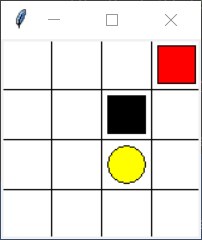
下面我们用一个具体的例子来演示DQN的应用，这里参考了Morvan的DQN的代码，建立了一个简易的4*4宫格的具有障碍的最短路径的游戏。该游戏非常简单，基本要求就是要控制方块在不触碰黑色方块的前提找到终点。在图中每个状态的可选择的动作最多有四个：上、下、左、右。进入黑色方块位置的奖励为-1，走到终点位置的奖励为1，其余位置的奖励均为0。

在此详细讲解代码的DQN算法核心部分，环境部分代码见：https://github.com/MorvanZhou/

class DeepQNetwork:
    def __init__(
            self,
            n_actions,#acttion space=4
            n_features,#features=state
            learning_rate=0.01,
            reward_decay=0.9,
            e_greedy=0.9,
            replace_target_iter=300,
            memory_size=500,#the size of memory bank
            batch_size=32,
            e_greedy_increment=None,
            output_graph=False,#tensorboard 输出神经网络架构
    ):
        self.n_actions = n_actions
        self.n_features = n_features
        self.lr = learning_rate
        self.gamma = reward_decay
        self.epsilon_max = e_greedy
        self.replace_target_iter = replace_target_iter
        self.memory_size = memory_size
        self.batch_size = batch_size
        self.epsilon_increment = e_greedy_increment
        self.epsilon = 0 if e_greedy_increment is not None else self.epsilon_max

        # total learning step
        self.learn_step_counter = 0

        # initialize zero memory [s, a, r, s_]#初始化经验池
        self.memory = np.zeros((self.memory_size, n_features * 2 + 2))

        # consist of [target_net, evaluate_net]
        self._build_net()
        t_params = tf.get_collection('target_net_params')
        e_params = tf.get_collection('eval_net_params')
        self.replace_target_op = [tf.assign(t, e) for t, e in zip(t_params, e_params)]

        self.sess = tf.Session()

        if output_graph:
            # $ tensorboard --logdir="logs/"
            # tf.train.SummaryWriter soon be deprecated, use following
            tf.summary.FileWriter("logs/", self.sess.graph)

        self.sess.run(tf.global_variables_initializer())
        self.cost_his = []

self.replace_target_op:表示Q-target网络要从Q-predict中复制神经网络的参数。

经验池（memory bank）中存放的数据样本为：当前状态，选择的动作，奖励，下一个状态

在该游戏中，状态的描述是通过16宫格中的二维的坐标来表示的，对应代码中的features。

 def _build_net(self):
        # ------------------ build evaluate_net ------------------
        self.s = tf.placeholder(tf.float32, [None, self.n_features], name='s')  # input
        self.q_target = tf.placeholder(tf.float32, [None, self.n_actions], name='Q_target')  # for calculating loss
        with tf.variable_scope('eval_net'):
            # c_names(collections_names) are the collections to store variables
            c_names, n_l1, w_initializer, b_initializer = \
                ['eval_net_params', tf.GraphKeys.GLOBAL_VARIABLES], 10, \
                tf.random_normal_initializer(0., 0.3), tf.constant_initializer(0.1)  # config of layers
#第一层网络的神经元个数为n_l1:10
            # first layer. collections is used later when assign to target net
            with tf.variable_scope('l1'):
                w1 = tf.get_variable('w1', [self.n_features, n_l1], initializer=w_initializer, collections=c_names)
                b1 = tf.get_variable('b1', [1, n_l1], initializer=b_initializer, collections=c_names)
                l1 = tf.nn.relu(tf.matmul(self.s, w1) + b1)
#l1层输入经过RELU激活函数，输出为[None,n_l1]

            # second layer. collections is used later when assign to target net
            with tf.variable_scope('l2'):
                w2 = tf.get_variable('w2', [n_l1, self.n_actions], initializer=w_initializer, collections=c_names)
                b2 = tf.get_variable('b2', [1, self.n_actions], initializer=b_initializer, collections=c_names)
                self.q_eval = tf.matmul(l1, w2) + b2
#l2输出层结果为：[None,self_action]，输出结果为Q-predict的值
        with tf.variable_scope('loss'):
            self.loss = tf.reduce_mean(tf.squared_difference(self.q_target, self.q_eval))
#采用Mean Square Error计算Q-predict和Q-target之间的误差
        with tf.variable_scope('train'):
            self._train_op = tf.train.RMSPropOptimizer(self.lr).minimize(self.loss)
#此处梯度下降采用RMSprop进行计算
        # ------------------ build target_net ------------------
        self.s_ = tf.placeholder(tf.float32, [None, self.n_features], name='s_')    # input
        with tf.variable_scope('target_net'):
            # c_names(collections_names) are the collections to store variables
            c_names = ['target_net_params', tf.GraphKeys.GLOBAL_VARIABLES]
#可以看到Q-target和Q-predict的网络结构完全相同，不同在于Q-target采用的参数是比较旧的，而Q-predcit采用的参数就是每次都会随着梯度计算更新。
            # first layer. collections is used later when assign to target net
            with tf.variable_scope('l1'):
                w1 = tf.get_variable('w1', [self.n_features, n_l1], initializer=w_initializer, collections=c_names)
                b1 = tf.get_variable('b1', [1, n_l1], initializer=b_initializer, collections=c_names)
                l1 = tf.nn.relu(tf.matmul(self.s_, w1) + b1)

            # second layer. collections is used later when assign to target net
            with tf.variable_scope('l2'):
                w2 = tf.get_variable('w2', [n_l1, self.n_actions], initializer=w_initializer, collections=c_names)
                b2 = tf.get_variable('b2', [1, self.n_actions], initializer=b_initializer, collections=c_names)
                self.q_next = tf.matmul(l1, w2) + b2

以上是DQN中重要的结构：采用了两个结构完全相同，但参数不同步更新的全连接神经网络作为Q-table的代替输出Q-target和Q-predict，两个全连接神经网络都只采用了一层的隐藏层，激活函数使用了RELU，结构非常简单。当然，这里也可以采用CNN作为神经网络的结构。

 def store_transition(self, s, a, r, s_):
        if not hasattr(self, 'memory_counter'):
            self.memory_counter = 0
#判断self对象有name特性返回True， 否则返回False。若没有这个索引值memory_counter，则令self.memory_counter=0
        transition = np.hstack((s, [a, r], s_))

        # replace the old memory with new memory
        index = self.memory_counter % self.memory_size
#总 memory 大小是固定的, 如果超出总大小, 取index为余数，旧 memory 就被新 memory 替换
        self.memory[index, :] = transition
#堆栈原理，在经验池中的数据遵循先进先出，后进后出的原则
        self.memory_counter += 1

   def choose_action(self, observation):
        # to have batch dimension when feed into tf placeholder
        observation = observation[np.newaxis, :]
#因为observation在传入时是一维的数值
#下面采取epsilon-greedy的策略
#当随机抽取数<0.9时，执行贪婪策略;当随机抽取数>0.9，则执行随机策略
        if np.random.uniform() < self.epsilon:
            # forward feed the observation and get q value for every actions
            actions_value = self.sess.run(self.q_eval, feed_dict={self.s: observation})
            action = np.argmax(actions_value)
        else:
            action = np.random.randint(0, self.n_actions)
        return 

以上两个函数是对经验池的填充和动作的选择。接下来就是对经验池中的经验进行回放以及更新Q-target网络参数。

    def learn(self):
        # check to replace target parameters
        if self.learn_step_counter % self.replace_target_iter == 0:
            self.sess.run(self.replace_target_op)
            print('\ntarget_params_replaced\n')
#判断是否对Q-target网络参数进行更新，更新后打印

        # sample batch memory from all memory
        if self.memory_counter > self.memory_size:
            sample_index = np.random.choice(self.memory_size, size=self.batch_size)
        else:
            sample_index = np.random.choice(self.memory_counter, size=self.batch_size)
        batch_memory = self.memory[sample_index, :]
#对经验池的一个简单判断，当counter计数大于经验池容量时，说明经验池已满，因此我们直接在经验池中取样即可。若相反，说明此时经验池还未满，我们则只能对已存储了的数据进行取样
        q_next, q_eval = self.sess.run(
            [self.q_next, self.q_eval],
            feed_dict={
                self.s_: batch_memory[:, -self.n_features:],  # fixed params
                self.s: batch_memory[:, :self.n_features],  # newest params
            })
#把取样传入神经网络中进行回放
        # change q_target w.r.t q_eval's action
        q_target = q_eval.copy()

        batch_index = np.arange(self.batch_size, dtype=np.int32)
        eval_act_index = batch_memory[:, self.n_features].astype(int)
        reward = batch_memory[:, self.n_features + 1]
# 这个相当于将q_target按[batch_index, eval_act_index]索引计算出相应位置的q—_target值
        q_target[batch_index, eval_act_index] = reward + self.gamma * np.max(q_next, axis=1)
#以下是莫烦本人的解释：
"""
        假如在这个 batch 中, 我们有2个提取的记忆, 根据每个记忆可以生产3个 action 的值:
        q_eval =
         [[1, 2, 3],
         [4, 5, 6]]
        q_target = q_eval =
        [[1, 2, 3],
         [4, 5, 6]]
        然后根据 memory 当中的具体 action 位置来修改 q_target 对应 action 上的值:
                            q_target[batch_index, eval_act_index] = reward + self.gamma * np.max(q_next, axis=1)
        比如在:
            记忆 0 的 q_target 计算值是 -1, 而且我用了 action 0;
            记忆 1 的 q_target 计算值是 -2, 而且我用了 action 2:
        q_target =
        [[-1, 2, 3],
         [4, 5, -2]]
        所以 (q_target - q_eval) 就变成了:
        [[(-1)-(1), 0, 0],
         [0, 0, (-2)-(6)]]
        """

在上图代码中的：change q_target w.r.t q_eval's action这一部分，实际上也是DQN网络中比较难理解的部分。在DQN中，我们拥有两个神经网络，假设我们在记忆中在Q-predict网络中选择了action1，其对应的Q值=3。根据DQN的Q值更新公式，在Q-target网络中我们是根据贪婪法则选择当前状态对应的Q值最大的action。这样就会出现一种情况，当在Q-predict中选择了action1，有可能对应的Q-target中，选择的Q值最大的action是action0。因此就出现了动作位置不对应的情况，这种情况就会出现两个选择的action，无法通过计算误差反向传播更新参数。因此这部分代码就是为了解决这种情况，无论在Q-target网络中Q值最大对应的action是什么，我们都将在Q-predict网络中选择的action对应到Q-target网络中。举个例子：

Q-predict=[0,-3,0]表示这一个记忆中选用了action1，action1的Q=-3，其他的Q均为0；

Q-target=[1,0,0]表示在这个记忆中的Q=reward+gamma*maxQ(s_)=1,但是在s_上我们选取了action0,此时两个action无法对应上，我们应该把Q-target的样本修改成：[0,1,0]，和Q-predict对应起来。

  _, self.cost = self.sess.run([self._train_op, self.loss],
                                     feed_dict={self.s: batch_memory[:, :self.n_features], self.q_target: q_target})
        self.cost_his.append(self.cost)  # 反向训练

        # increasing epsilon提高选择正确的概率，直到self.epsilon_max
        self.epsilon = self.epsilon + self.epsilon_increment if self.epsilon < self.epsilon_max else self.epsilon_max
        self.learn_step_counter += 1

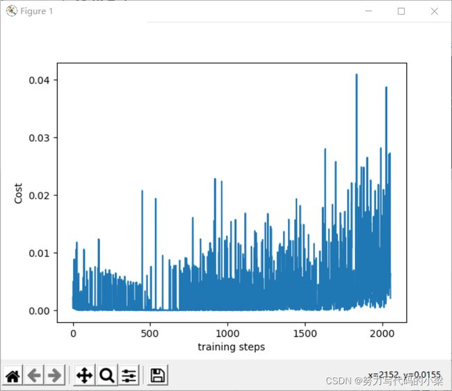
    def plot_cost(self):  # 展示学习曲线
        import matplotlib.pyplot as plt
        plt.plot(np.arange(len(self.cost_his)), self.cost_his)  # arange函数用于创建等差数组，arange返回的是一个array类型的数据
        plt.ylabel('Cost')
        plt.xlabel('training steps')
        plt.show()

以下是代码运行后的游戏过程图和学习曲线：

 

 tensorboard输出结果：

参考资料：

https://www.cnblogs.com/pinard/p/9756075.htmlhttps://blog.csdn.net/november_chopin/article/details/107912720

https://zhuanlan.zhihu.com/p/46852675

https://icml.cc/2016/tutorials/deep_rl_tutorial.pdf

https://ojs.aaai.org/index.php/AAAI/article/view/10295

以上是本教程全部内容，有问题欢迎大家在评论区里交流！