Nilearn：绘制大脑图像

文章来源于微信公众号（茗创科技），欢迎有兴趣的朋友搜索关注。

Nilearn简介

Nilearn使许多先进的机器学习、模式识别和多元统计技术在神经成像数据上的应用变得很容易，如MVPA(Mutli-Voxel pattern Analysis)、解码、预测建模、功能连接、大脑分割、连接体。Nilearn可以很容易地用于任务态和静息态fMRI，或者VBM数据。Nilearn的价值可以被看作是特定领域的特征工程构建，也就是说，将神经成像数据塑造成一个非常适合统计学习的特征矩阵。此外，nilearn具有绘图功能，能够可视化神经成像的像和头表。这里主要给大家介绍的是如何用nilearn绘制大脑图像。在开始使用nilearn绘制大脑图像之前，先来了解nilearn在不同系统中的安装。

Nilearn安装

在Windows系统中

①下载并安装64位Anaconda (https://www.anaconda.com/products/distribution)。建议安装一个完整的64位科学Python发行版，比如Anaconda。因为它满足Nilearn的所有要求，也能节省时间和避免不必要的麻烦。Nilearn需要安装Python和以下依赖项：ipython、scipy、scikit-learn、joblib、matplotlib、nibabel和pandas。

②打开命令提示符。(按“Win-R”，输入“cmd”，然后按“Enter”。这将打开程序cmd.exe，这是命令提示符)。然后输入pip install -U --user nilearn，并按“Enter”键。

③打开IPython。(可以在命令提示符中输入“ipython”并按“Enter”打开)。然后输入In [1]: import nilearn，并按“Enter”。

注：如果没有提示出现错误，说明已经正确安装了Nilearn。

在Mac系统中

①同样下载并安装64位Anaconda。

②打开一个Terminal。(选择Applications--Utilities，双击Terminal)，然后输入pip install -U --user nilearn，并按“Enter”键。

③打开IPython。(可以在Terminal中输入“ipython”并按“Enter”键打开)。然后输入In [1]: import nilearn，并按“Enter”。

注：如果没有提示出现错误，说明已经正确安装。

绘制大脑图像

①不同的绘图函数：Nilearn有一组绘图函数，可以根据特定的应用来绘制大脑的像(volumes)。此外，还可以使用不同的方法来寻找脑切割坐标。

plot_anat：用函数plot_anat绘制解剖图像。如可视化haxby数据集解剖图像。

plotting.plot_anat(haxby_anat_filename, title="plot_anat")

plot_epi：用函数plot_epi绘制EPI或T2*图像。

# 导入图像处理工具
from nilearn import image
# 计算函数图像的voxel_wise平均值
# 将函数图像从4D降维至3D
mean_haxby_img = image.mean_img(haxby_func_filename)
# 可视化均值图像(3D)
plotting.plot_epi(mean_haxby_img, title="plot_epi")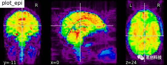

plot_glass_brain：绘制玻璃脑图像。默认情况下，plot_glass_brain使用一种名为'ortho'的显示模式，它会产生三个投影，等价于在plot_glass_brain中指定display_mode='ortho'。

from nilearn import plotting
from nilearn.plotting import plot_glass_brain
# 整个大脑的矢状切面和地图的阈值是3
plot_glass_brain(stat_img, threshold=3)

plot_stat_map：绘制统计图像，如T图、Z图或ICA。

from nilearn import plotting
# 在EPI模板上手动可视化t-map图像
# 使用给定的cut_coords定位坐标
plotting.plot_stat_map(stat_img,
                       threshold=3, title="plot_stat_map",
cut_coords=[36, -27, 66])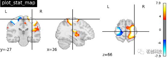

plot_roi：用可选的背景绘制ROI或掩膜。如将haxby数据集上的腹侧颞区图像可视化，并将坐标自动定位于感兴趣区域(roi)。

plotting.plot_roi(haxby_mask_filename, bg_img=haxby_anat_filename,
                  title="plot_roi")

plot_connectome：绘制连接体图像。使用函数nilearn.plot .plot_connectome来显示连接图。

from nilearn import plotting

plotting.plot_connectome(partial_correlation_matrix, dmn_coords,
                         title="Default Mode Network Connectivity")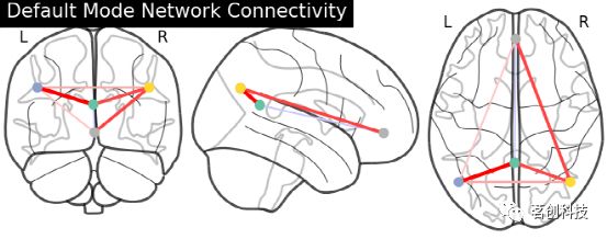

显示脑半球投射的连接体。注意(0,-52,18)包含在两个大脑半球中，因为x==0。

from nilearn import plotting

plotting.plot_connectome(partial_correlation_matrix, dmn_coords,
                         title="Default Mode Network Connectivity")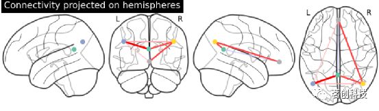

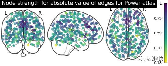
plot_markers：绘制网络节点。根据所提供的节点测量(即连接强度)，自动绘制网络节点并对其进行颜色编码，如在不同参考图集上比较连接体。

# 计算每个节点的归一化绝对强度
node_strength = np.sum(np.abs(matrix), axis=0)
node_strength /= np.max(node_strength)

plotting.plot_markers(
    node_strength,
    coords,
    title='Node strength for absolute value of edges for Power atlas',
)

plot_carpet：绘制随时间变化的体素强度。

import matplotlib.pyplot as plt
from nilearn.plotting import plot_carpet
display = plot_carpet(adhd_dataset.func[0], mask_img, t_r=t_r)
display.show()

设置不同的显示模式

Nilearn主要是根据参数display_mode和cut_coords来设置大脑图像的不同显示模式。参数display_mode用于沿着给定的特定方向绘制大脑层，方向包括'ortho'，'tile'，'mosaic'，'x'，'y'，'z'，'yx'，'xz'，'yz'。而参数cut_coords用于指定有限数量的层，以便沿着给定层的方向进行可视化。参数cut_coords也可以根据特定层的方向在MNI空间中给出其特定坐标。这有助于我们指出大脑层的特定激活位置。

用给定的坐标在“矢状面”、“冠状面”和“轴位”中进行可视化。设置Display_mode= 'ortho'， cut_cocord=[36, -27, 60]，Ortho slicer表示沿x，y，z方向进行3次切割。

plotting.plot_stat_map(stat_img, display_mode='ortho',
                       cut_coords=[36, -27, 60],
                       title="display_mode='ortho', cut_coords=[36, -27, 60]")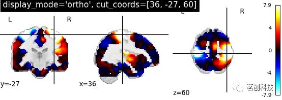

对于轴位可视化，设置display_mode='z'，cut_coords=5时，表示在z方向上切割，指定切割的次数。

plotting.plot_stat_map(stat_img, display_mode='z', cut_coords=5,
                       title="display_mode='z', cut_coords=5")

对于矢状面可视化，设置display_mode='x'，cut_coords=[-36, 36]时，表示在x方向上切割，指定精确的切割。

plotting.plot_stat_map(stat_img, display_mode='x',
                       cut_coords=[-36, 36],
                       title="display_mode='x', cut_coords=[-36, 36]")

对于冠状面可视化，设置display_mode= 'y'，cut_coords=1，表示在y方向进行切割，只切割1次，即自动定位。

plotting.plot_stat_map(stat_img, display_mode='y', cut_coords=1,
                       title="display_mode='y', cut_coords=1")

设置display_mode= 'z'，cut_coords=1，colorbar= False，表示在z方向切割，只切割1次，即自动定位，而且不呈现颜色条。

plotting.plot_stat_map(stat_img, display_mode='z',
                       cut_coords=1, colorbar=False,
                       title="display_mode='z', cut_coords=1, colorbar=False")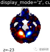

设置display_mode= 'xz'，cut_coords=[36, 60]，表示在x和z方向上进行切割，并且是手动定位切割。

plotting.plot_stat_map(stat_img, display_mode='xz',
                       cut_coords=[36, 60],
                       title="display_mode='xz', cut_coords=[36, 60]")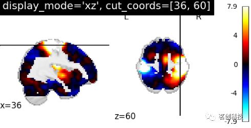

设置display_mode= 'yx'，cut_coords=[-27, 36]，表示在y和x方向上切割，手动定位。

plotting.plot_stat_map(stat_img, display_mode='yx',
                       cut_coords=[-27, 36],
                       title="display_mode='yx', cut_coords=[-27, 36]")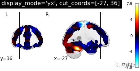

设置display_mode= 'yz'，cut_coords=[-27, 60]，表示在y和z方向上切割，手动定位。

plotting.plot_stat_map(stat_img, display_mode='yz',
                       cut_coords=[-27, 60],
                       title="display_mode='yz', cut_coords=[-27, 60]")

设置display_mode= 'tiled'，cut_coords=[36, -27, 60]，Tiled slicer表示沿着x, y, z方向进行3次切割，以2×2的网格进行排列。

plotting.plot_stat_map(stat_img, display_mode='tiled',
                       cut_coords=[36, -27, 60],
                       title="display_mode='tiled'")

设置display_mode= 'mosaic'，Mosaic slicer表示沿x, y, z方向进行多次切割，默认自动定位切割。

plotting.plot_stat_map(stat_img, display_mode='mosaic',
                       title="display_mode='mosaic' default cut_coords")

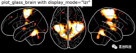
玻璃脑绘制：设置display_mode= 'lzr'。

plot_glass_brain(
    stat_img, title='plot_glass_brain with display_mode="lzr"',
    black_bg=True, display_mode='lzr', threshold=3
)

玻璃脑绘制：设置display_mode='lyrz'。

plot_glass_brain(
    stat_img, threshold=0, colorbar=True,
    title='plot_glass_brain with display_mode="lyrz"',
    plot_abs=False, display_mode='lyrz'
)

添加边缘，轮廓线，轮廓填充，标记，比例尺

display.add_edges (img)：添加图像的边缘。

# 导入图像处理工具进行脑功能图像的基本处理
from nilearn import image

mean_haxby_img = image.mean_img(haxby_func_filename)
display = plotting.plot_anat(mean_haxby_img, title="add_edges")
display.add_edges(haxby_anat_filename, color='r')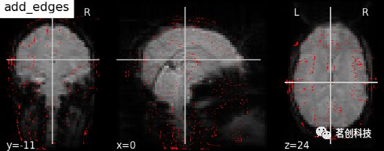

display.add_contours(img, levels=[.5], colors=' r ')：添加轮廓线。

display = plotting.plot_anat(mean_haxby_img, title="add_contours",
                             cut_coords=[-34, -39, -9])

display.add_contours(haxby_mask_filename, levels=[0.5], colors='r')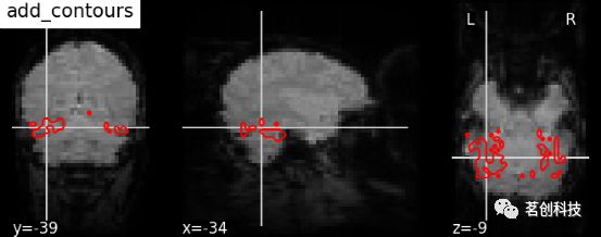

display.add_contours(img, filled=True, alpha=0.7, levels=[0.5], colors=' b ')：轮廓填充。

display = plotting.plot_anat(mean_haxby_img,
                             title="add_contours with filled=True",
cut_coords=[-34, -39, -9])

display.add_contours(haxby_mask_filename, filled=True, alpha=0.7,
levels=[0.5], colors='b')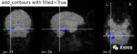

display.add_markers(coords, marker_color=' y ', marker_size=100)：添加标记。

display = plotting.plot_anat(mean_haxby_img, title="add_markers",
                             cut_coords=[-34, -39, -9])
coords = [(-34, -39, -9)]
display.add_markers(coords, marker_color='y', marker_size=100)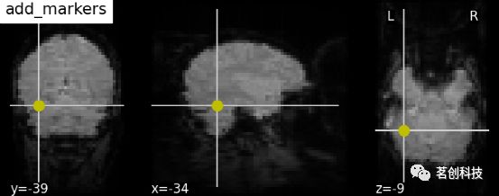

display.annotate(scalebar=True)：添加比例尺。

display = plotting.plot_anat(mean_haxby_img,
                             title="adding a scale bar",
                             cut_coords=[-34, -39, -9])
display.annotate(scalebar=True)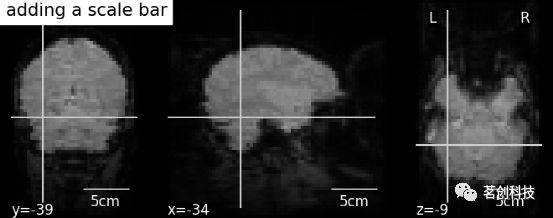

# 进一步的设置可以通过scale_*关键字参数来实现。例如，将单位更改为mm，或者使用不同的比列尺大小
display = plotting.plot_anat(mean_haxby_img,
                             title="adding a scale bar",
                             cut_coords=[-34, -39, -9])
display.annotate(scalebar=True, scale_size=25, scale_units='mm')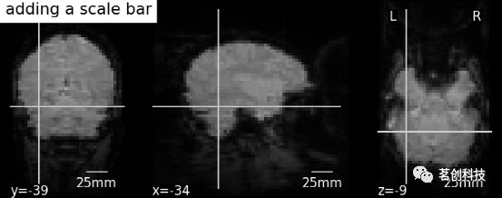

显示或保存到一个图像文件

要在运行脚本时显示图形，需要调用nilearn.plot.show(这是matplotlib.pyplot.show的别名)：

from nilearn import plotting
plotting.show()

从绘图函数中输出图像文件的最简单方法是指定output_file参数：

from nilearn import plotting
plotting.plot_stat_map(img, output_file='pretty_brain.png')

​​​​​​​使用savefig方法将绘制好的图像保存为图像文件：

from nilearn import plotting
display = plotting.plot_stat_map(img)    
display.savefig('pretty_brain.png')    
display.close()

表面图像绘制

plot_surf_roi：绘制大脑表面图集

from nilearn import datasets
destrieux_atlas = datasets.fetch_atlas_surf_destrieux()
# 加载左脑图谱数据
parcellation = destrieux_atlas['map_left']
fsaverage = datasets.fetch_surf_fsaverage()
# fsaaverage数据集包含指向文件位置的文件名
print('Fsaverage5 pial surface of left hemisphere is at: %s' %
      fsaverage['pial_left'])
print('Fsaverage5 inflated surface of left hemisphere is at: %s' %
      fsaverage['infl_left'])
print('Fsaverage5 sulcal depth map of left hemisphere is at: %s' %
      fsaverage['sulc_left'])

# 可视化
from nilearn import plotting
plotting.plot_surf_roi(fsaverage['pial_left'], roi_map=parcellation,
                       hemi='left', view='lateral',
                       bg_map=fsaverage['sulc_left'], bg_on_data=True,
                       darkness=.5)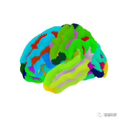

# 在fsaverage5表面显示Destrieux分割
plotting.plot_surf_roi(fsaverage['infl_left'], roi_map=parcellation,
                       hemi='left', view='lateral',
                       bg_map=fsaverage['sulc_left'], bg_on_data=True,
                       darkness=.5)

# 以不同视角显示Destrieux分割：后部
plotting.plot_surf_roi(fsaverage['infl_left'], roi_map=parcellation,
                       hemi='left', view='posterior',
                       bg_map=fsaverage['sulc_left'], bg_on_data=True,
                       darkness=.5)

# 腹侧
plotting.plot_surf_roi(fsaverage['infl_left'], roi_map=parcellation,
                       hemi='left', view='ventral',
                       bg_map=fsaverage['sulc_left'], bg_on_data=True,
                       darkness=.5)
plotting.show()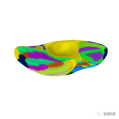

plot_surf_stat_map：绘制大脑表面的种子连接

# 读取数据
# 来自nilearn的NKI静息态数据
from nilearn import datasets
nki_dataset = datasets.fetch_surf_nki_enhanced(n_subjects=1)
print(('Resting state data of the first subjects on the '
       'fsaverag5 surface left hemisphere is at: %s' %
      nki_dataset['func_left'][0]))
# 左脑fsaverage5区Destrieux分割
destrieux_atlas = datasets.fetch_atlas_surf_destrieux()
parcellation = destrieux_atlas['map_left']
labels = destrieux_atlas['labels']
# Fsaverage5表面模板
fsaverage = datasets.fetch_surf_fsaverage()
# fsaaverage数据集包含指向文件位置的文件名
print('Fsaverage5 pial surface of left hemisphere is at: %s' %
      fsaverage['pial_left'])
print('Fsaverage5 inflated surface of left hemisphere is at: %s' %
      fsaverage['infl_left'])
print('Fsaverage5 sulcal depth map of left hemisphere is at: %s' %
      fsaverage['sulc_left'])

# 提取种子的时间序列
# 从nilearn加载静息态时间序列
from nilearn import surface
timeseries = surface.load_surf_data(nki_dataset['func_left'][0])
# 通过标签提取种子区域
pcc_region = b'G_cingul-Post-dorsal'
import numpy as np
pcc_labels = np.where(parcellation == labels.index(pcc_region))[0]
# 从种子区域提取时间序列
seed_timeseries = np.mean(timeseries[pcc_labels], axis=0)

# 计算基于种子的功能连接
# 计算种子时间序列与半球所有皮层节点时间序列之间的皮尔逊积矩相关系数
from scipy import stats
stat_map = np.zeros(timeseries.shape[0])
for i in range(timeseries.shape[0]):
    stat_map[i] = stats.pearsonr(seed_timeseries, timeseries[i])[0]
stat_map[np.where(np.mean(timeseries, axis=1) == 0)] = 0

# 在表面显示ROI
# 在ROI图中转换ROI指标
pcc_map = np.zeros(parcellation.shape[0], dtype=int)
pcc_map[pcc_labels] = 1

from nilearn import plotting
plotting.plot_surf_roi(fsaverage['pial_left'], roi_map=pcc_map,
                       hemi='left', view='medial',
                       bg_map=fsaverage['sulc_left'], bg_on_data=True,
                       title='PCC Seed')

参考来源：

https://nilearn.github.io/stable/plotting/index.html#interactive-plots

https://github.com/nilearn/nilearn/blob/9ddfa7259/nilearn/plotting/img_plotting.py#L414

https://nilearn.github.io/stable/auto_examples/01_plotting/plot_demo_more_plotting.html

文章来源于微信公众号（茗创科技），欢迎有兴趣的朋友搜索关注。