matlab pcolor怎么画多层的图,求助listDensityPlot，跟matlab的pcolor函数画出来的不一样...

该楼层疑似违规已被系统折叠 隐藏此楼查看此楼

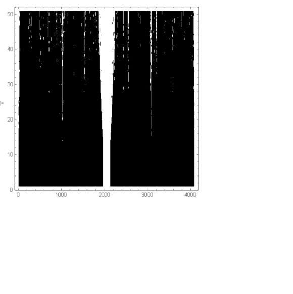
模拟一个光传播过程，代码如下，请问我用matlab算的热图跟MMA算的为啥不一样啊 MMA特别难看，见附图

Clear["Global`*"]

SetDirectory[NotebookDirectory[]]

"C:\\Users\\Tiny\\Desktop\\Mei_波导NLSE"

c = 3 10^8;

(*Generate time axis*)

N1 = 2^12;

\[ScriptCapitalS][x_] :=

Join[Take[x, -(Length[x]/2)], Take[x, Length[x]/2]];

tw = 50 10^-12;

fs = 10^-15;

ps = 10^-12;

mm = 1 10^-3;

nm = 10^-9;

um = 10^-6;

dt = tw/N1 // N;

t = Table[x, {x, -N1/2 dt, (N1/2 - 1) dt, dt}];

(*Generate frequency axis*)

\[Omega] = (2 \[Pi])/tw Table[x, {x, -(N1/2), N1/2 - 1, 1}] //

N // \[ScriptCapitalS];

k = \[Omega];

k2 = k^2;

k3 = k^3;

kTHz = (k/2/\[Pi]*10^-12) // \[ScriptCapitalS];

d\[Omega] = \[Omega][[2]] - \[Omega][[1]];

df = d\[Omega]/(2 \[Pi]);

\[Lambda]0 = 1550 nm;

f0 = c/\[Lambda]0;

\[Omega]0 = 2 \[Pi] f0;

\[Lambda] = (2 \[Pi] c)/(\[Omega]0 + \[Omega]) // N;

\[Lambda]1 = \[ScriptCapitalS][\[Lambda]];

(*Nonlinear parameters*)

\[Gamma]0 = 76.74348226;

\[Beta]20 = 1.471954 ps^2;

(*Raman parameters*)

fR = 0.043;

\[Tau]1 = 10 fs;

\[Tau]2 = 3 ps;

\[Omega]R = 15.6 1 10^12 2 \[Pi];

hR = Table[0 x, {x, 1, N1, 1}];

hR = Join[Table[0, {t, -N1/2 , 0, 1}],

Table[\[Omega]R^2 \[Tau]1 Exp[(-t/\[Tau]2)] Sin[t/\[Tau]1], {t,

dt, (N1/2 - 1) dt, dt}]];

hRNorm = hR // Total;

RTf = (N1 Fourier[hR // \[ScriptCapitalS],

FourierParameters -> {-1, 1}])/hRNorm ;

(*Pulse parameters*)

T0 = 200 fs/1.665;

P0 = 2.2;

Phase = 0;

alpha = 0/4.343;

g = 225;

a1 = -4.6147 10^11;

b1 = 1.2421 10^10;

c1 = -8.6932 10^7;

d1 = -5.6924 10^5;

e1 = 1.2566 10^4;

f1 = 7.6686 10^1;

a2 = 6.4523 10^-15;

b2 = -2.2439 10^-16;

c2 = 2.8207 10^-18;

d2 = -1.0267 10^-20;

e2 = -1.1107 10^-22;

f2 = 1.4719 10^-24;

(* Initial pulse *)

z = 0;

At = Table[

P0^(1/2) Exp[-(t/T0)^2/2] Exp[1 I Phase*t^2/(2 T0^2)], {t, -N1/

2 dt, (N1/2 - 1) dt, dt}];

ListPlot[{t, At} // Transpose, PlotRange -> All, Joined -> True,

Frame -> True, Axes -> False];

Aw0 = (Fourier[At] // \[ScriptCapitalS] // Abs)^2;

Aw0max = Max[Aw0];

Aw0N = Aw0/Aw0max;

At0 = (At // Abs)^2;

At0N = Abs[At]^2/P0;

ListPlot[{t/ps, At0N} // Transpose, Joined -> True, Frame -> True,

PlotRange -> All,

FrameLabel -> {Style["Time(ps)", 10, Red],

Style["Normalized Intensity", 10, Red]}]

ListPlot[{\[Lambda]1/nm, Aw0N} // Transpose, Joined -> True,

Frame -> True, PlotRange -> All,

FrameLabel -> {Style["Wavelength(nm)", 10, Red],

Style["Normalized Intensity", 10, Red]}]

(*Initialize the marks*)

Pf = (At // Fourier // \[ScriptCapitalS] // Abs)^2;

(*Propagation in the fiber*)

Umh = {};

Umhw = {};

Amh = {};

T = {};

dz = 0.2 mm;

L = 10 mm;

For[i = 0, i <= L/dz, i++;

Umh = Append[Umh, Abs[At]^2];

Umhw = Append[Umhw, Abs[At // Fourier // \[ScriptCapitalS]]^2];

Amh = Append[Amh, At];

gammaz = a1*z^5 + b1*z^4 + c1*z^3 + d1*z^2 + e1*z + f1;

gammazh2 =

a1*(z + dz/2)^5 + b1*(z + dz/2)^4 + c1*(z + dz/2)^3 +

d1*(z + dz/2)^2 + e1*(z + dz/2) + f1;

gammazh =

a1*(z + dz)^5 + b1*(z + dz)^4 + c1*(z + dz)^3 + d1*(z + dz)^2 +

e1*(z + dz) + f1;

beta2z = a2*z^5 + b2*z^4 + c2*z^3 + d2*z^2 + e2*z + f2;

beta2zh2 =

a2*(z + dz/2)^5 + b2*(z + dz/2)^4 + c2*(z + dz/2)^3 +

d2*(z + dz/2)^2 + e2*(z + dz/2) + f2;

beta2zh =

a2*(z + dz)^5 + b2*(z + dz)^4 + c2*(z + dz)^3 + d2*(z + dz)^2 +

e2*(z + dz) + f2;

beta2zsum =

a2*z^6/6 + b2*z^5/5 + c2*z^4/4 + d2*z^3/3 + e2*z^2/2 + f2*z;

beta2zh2sum =

a2*(z + dz/2)^6/6 + b2*(z + dz/2)^5/5 + c2*(z + dz/2)^4/4 +

d2*(z + dz/2)^3/3 + e2*(z + dz/2)^2/2 + f2*(z + dz/2);

beta2zhsum =

a2*(z + dz)^6/6 + b2*(z + dz)^5/5 + c2*(z + dz)^4/4 +

d2*(z + dz)^3/3 + e2*(z + dz)^2/2 + f2*(z + dz);

(*RK4*)

Lz = -0.5*alpha*z + 1 I*0.5*beta2zsum*k2;

Af0 = Fourier[At]*Exp[-Lz];

(*K1*)

Pt = Abs[At]^2;

Ramant = Pt;

dAf1 = I*gammaz*Exp[-Lz]*Fourier[Ramant*At];

(*K2*)

(*Dispersion*)

Lz = -0.5*alpha*(z + dz/2) + 1 I*0.5*beta2zh2sum*k2;

At = Fourier[Exp[Lz]*(Af0 + dAf1*dz/2)];

bb = Exp[Lz];

bb1 = (Af0 + dAf1*dz/2);

(*Raman and other nonlinear effect*)

Pt = Abs[At]^2;

Ramant = Pt;

dAf2 = 1 I*gammazh2*Exp[-Lz]*Fourier[Ramant*At];

(*K3*)

(*Dispersion*)

Lz = -0.5*alpha*(z + dz/2) + 1 I*0.5*beta2zh2sum*k2;

At = Fourier[Exp[Lz]*(Af0 + dAf2*dz/2)];

(*Raman and other nonlinear effect*)

Pt = Abs[At]^2;

Ramant = Pt;

dAf3 = 1 I*gammazh2*Exp[-Lz]*Fourier[Ramant*At];

(*K4*)

(*Dispersion*)

Lz = -0.5*alpha*(z + dz) + 1 I*0.5*beta2zhsum*k2;

At = Fourier[Exp[Lz]*(Af0 + dAf3*dz)];

(*Raman and other nonlinear*)

Pt = Abs[At]^2;

Ramant = Pt;

dAf4 = 1 I*gammazh*Exp[-Lz]*Fourier[Ramant*At];

(*Final step*)

Af = Af0 + dz/6*(dAf1 + 2*dAf2 + 2*dAf3 + dAf4);

At = Fourier[Exp[Lz]*Af];

Pf = Abs[\[ScriptCapitalS][Exp[Lz]*Af]]^2;

(*End of RK4*)

z = z + dz;

]

At1 = Abs[At]^2;

At1N = Abs[At]^2/P0;

P0 = ListPlot[{t, At1N} // Transpose, PlotRange -> All, Frame -> True,

Axes -> False, Joined -> True,

FrameLabel -> {Style["Delay(ps)", 12, Red],

Style["Intensity", 12, Red]}];

P1 = ListPlot[{\[Lambda]1/um,

Abs[Fourier[At]]^2 // \[ScriptCapitalS]} // Transpose,

PlotRange -> {{1.3, 1.8}, {0, 1}}, PlotRange -> All, Frame -> True,

Axes -> False, Joined -> True,

FrameLabel -> {Style["Wavelength (um)", 12, Red],

Style["Spectrum (a.u.)", 12, Red]}];

P2 = ListPlot[{\[Lambda]1/um, Aw0} // Transpose,

PlotRange -> {{1.3, 1.8}, {0, 1}}, Frame -> True, Axes -> False,

Joined -> True,

FrameLabel -> {Style["Wavelength (um)", 12, Red],

Style["Spectrum (a.u.)", 12, Red]}, PlotStyle -> {Red, Dashed}];

Show[P1, P2]

ListDensityPlot[Umh/Max[Umh], ColorFunction -> "SunsetColors"]