【CV-baseline】02VGG-论文笔记

论文标题：Very deep convolutional networks forlarge-scale image recognition（大规模图像识别的深度卷积神经网络）
论文作者: Karen Simonyan & Andrew Zisserman
单位:VGG(牛津大学视觉几何组)
发表会议及时间:ICLR 2015

学习目标

1. 模型结构设计
   1. 小卷积核
   2. 堆叠使用卷积核
   3. 分辨率减半，通道数翻倍
2. 训练技巧
   1. 尺度扰动
   2. 预训练模型初始化
3. 测试技巧
   1. 多尺度测试
      1. Dense测试
      2. Multi-crop测试
   2. 多模型融合

论文导读

背景、成果和意义

背景

1. ILSVRC-2014

2. 相关研究

   • AlexNet: 借鉴卷积模型结构

   • ZFNet: 借鉴其采用小卷积核思想

   • OverFeat: Dense test, 借鉴全卷积，实现了高效的稠密预测

     • 重复使用中间像素

     • 多重feature map提高了分辨率

   • NIN：尝试$1\times 1$卷积

成果

1. ILSVRC定位冠军，分类亚军
2. 开源VGG16， VGG19.

意义

1. 开启小卷积核，$3\times 3$卷积核成为主流模型
2. 深度卷积模型时代。 作为各类图像任务的骨干网络结构:分类、定位、检测、分割一系列图像任务大都有VGG为骨干网络的尝试

论文泛读

摘要

1. 本文主题:在大规模图像识别任务中，探究卷积网络深度对分类准确率的影响
2. 主要工作:研究3*3卷积核增加网络模型深度的卷积网络的识别性能，同时将模型加深到16-19层
3. 本文成绩:VGG在ILSVRC-2014获得了定位任务冠军和分类任务亚军
4. 泛化能力:VGG不仅在ILSVRC获得好成绩，在别的数据集中表现依旧优异
5. 开源贡献:开源两个最优模型，以加速计算机视觉中深度特征表示的进一步研究

越靠后的卷积层利用非线性更强的操作，后面的卷积核数量更多

VGG结构

文中展示了总共六种模型：A, A-LRN, B, C, D, E

(论文table1)

模型共性:

1. 5个maxpool
2. maxpool之后，特征图通道数翻倍直至512
3. 3个FC层进行分层输出
4. maxpool之间采用多个卷积层堆叠，对特征进行提取和抽象
5. 都是从11层权重层(weight layers)开始堆叠。借鉴Goodfellow的论文(Goodfellow et al. (2014) applied deep ConvNets (11 weight layers) to the task of street number recognition)

演变过程

1. A:11层卷积
2. A-LRN:基于A增加一个LRN
3. B: 第1，2个block中增加1个卷积33卷积
4. C: 第3， 4， 5个block分别增加1个$1\times 1$卷积， 表明增加非线性有益于指标提升
5. D:第3， 4， 5个block的$1\times 1$卷积替换为$3\times 3$，
6. E: 第3， 4， 5个block再分别增加1个$3\times 3$卷积

参数量对比

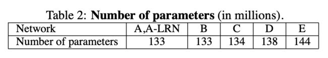
(论文table2)

VGG16 结构

网络层参数细节

网络层维度

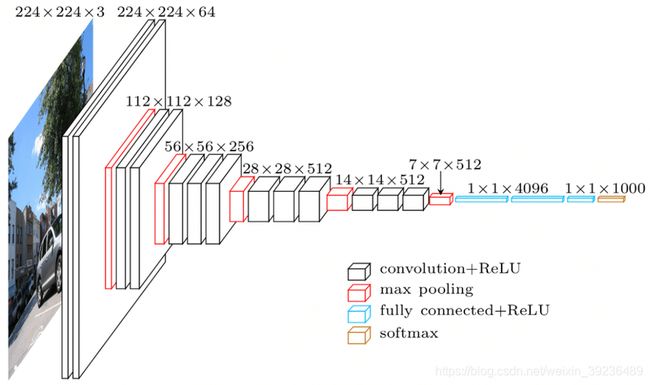
这里经历了5次maxpool，就意味着输入张量(假设$224\times 224$)的宽和高的维度减半了5次，所以最后的输出维度是
$$\frac{224}{2^5}=7$$
也就是图中$7\times 7\times 512$，然后flatten成一个$1\times 25088$维度的向量，连接后面的4096

【VGG-16和VGG-19差别在哪？
答：VGG 中定义了6种模型结构A~E，C模型 和D 模型都包含16 个权重层，其中C 模型是在第7 个卷积层使用$1\times 1$的卷积核，第3，4，5个block分别增加1层$1\times 1$卷积，作者使用$1\times 1$卷积核是为了增加模型的非线性，提升模型指标；D 模型将3，4，5个block的$1\times 1$卷积核替换为$3\times 3$卷积核，D模型和C模型 卷积核的数量都相等，现在pytorch 的官方定义的VGG 16 的模型中是D模型结构；E模型即VGG19,相比D模型和C模型，在第3，4，5个block再分别增加1层3*3卷积, 分别为conv3-256、conv3-512、conv3-512】

VGG 特点

堆叠$3\times 3$卷积核

增大感受野

2个$3\times 3$堆叠等价于1个$5\times 5$

(图片来源: https://www.jeremyjordan.me/convnet-architectures/)

3个$3\times 3$堆叠等价于1个$7\times 7$

其他作用

1. 增加非线性激活函数，增强了特征抽象能力
2. 减少了训练参数
3. 可看成$7\times 7$卷积核的正则化，强迫$7\times 7$分解为$3\times 3$

例子：假设输入，输出通道均为C个通道

一个$7\times 7$卷积核所需的参数量: $7\times 7\times C\times C=49C^2$,3个$3\times 3$卷积核所需参数量为$3\times 3\times 3\times C\times C=27C^2$。参数量减少$(49-27)27\approx 44\%$

尝试$1\times 1$卷积

借鉴NIN，引入利用$1\times 1$卷积， 增加非线性激活函数，提升模型效果

训练技巧

数据增强: Scale jittering

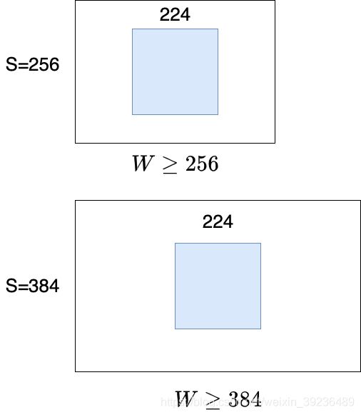
方法一：针对位置

训练阶段

1. 按比例缩放图片至最小边为S
2. 随机位置裁剪出$224\times 224$区域
3. 随机进行水平翻转

方法二：

修改RGB通道的像素值，实现颜色扰动

S设置方法

1. 固定值：S=256, 或者S=384
2. 随机值：每个batch的S在[256, 512]间随机选取，实现尺度扰动

预训练模型初始化

深度神经网络对初始化敏感

1. 深度加深时，用浅层网络初始。 B，C，D，E用A模型初始化

2. Multi-scale训练时，用小尺度初始化：

   1. S=384时，用S=256模型初始化
   2. S=[256, 512]时，用S=384模型初始化

3. 直接用Xavier初始化是现在的主流

测试技巧

多尺度测试

图片等比例缩放至最短边为Q。本文设置了3个Q，对图片进行预测，然后取平均

方法一：

S为固定值时， $Q=[\mathrm{S}-32,\mathrm{S},\mathrm{S}+32]$.比如S=256， Q=[224, 256, 288]

方法二：

S为随机值([256, 512])时， $Q=\left(S_{min},0.5\times \left(S_{min}+S_{max}\right),S_{max}\right)=(256,384,512)$

稠密测试(Dense test)

将FC层转换为卷积操作，变为全卷积网络，实现任意尺寸图片输入

1. 输入图片经过全卷积网络得到$N\times N\times 1000$特征图
2. 在通道维度($N\times N$)上求和(sum pool)计算平均值，得到$1\times 1000$输出向量

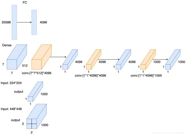
上图中的例子，如果原先训练时的S=256， 裁剪后的输入图片尺寸是224，那么如果Q=224输出的就是一个$1\times 1\times 1000$的张量。如果Q=448，那么，就得到一个$2\times 2\times 1000$的张量， 那么我们就要在通道维度上求和计算平均值得到一个$1\times 1\times 1000$的输出向量。

multi-crop测试

借鉴AlexNet与GoogLeNet，对图片进行Multi-crop，裁剪大小为$224\times 224$，并水平翻转 1张图，缩放至3种尺寸，然后每种尺寸裁剪出50张图片;$50=5\times 5\times 2$。那么总共三个Q值就有150张图片

因此测试分为两个steps

1. Step1： 等比例蒜放图像至Q1, Q2, Q3三种尺寸
2. Step2: 分别用三种方法
   1. Dense:全卷积，sum pool，得到$1\times 1000$
   2. Multi-crop:多个位置裁剪224*224区域
   3. Multi-crop & Dense:综合取平均

实验结果及分析

single scale evaluation

S为固定值时:Q = S， S为随机值时:$Q=0.5(S_{min}+S_{max})$

结论

1. 误差随深度加深而降低，当模型到达19层时，误差饱和，不再下降

2. 增加$1\times 1$有助于性能提升

3. 训练时加入尺度扰动，有助于性能

   提升

4. B模型中，$3\times 3$替换为$5\times 5$卷积，top1下降7%

multi-scale evaluation

方法一：

S为固定值时， $Q=[\mathrm{S}-32,\mathrm{S},\mathrm{S}+32]$.比如S=256， Q=[224, 256, 288]

方法二：

S为随机值([256, 512])时， $Q=\left(S_{min},0.5\times \left(S_{min}+S_{max}\right),S_{max}\right)=(256,384,512)$

结论：

1. 测试时采用Scale jittering有助于性能提升

multi-crop evaluation

方法: 等步长的滑动$224\times 224$的窗口进行裁剪，在尺 度为Q的图像上裁剪$5\times 5=25$张图片，然后再进 行水平翻转，得到50张图片，结合三个Q值， 一张图片得到150张图片输入到模型中

结论:

1. mulit-crop优于dense
2. multi-crop结合dense，可形成互补，达到最优结果

convnet confusion

方法: ILSVRC中，多模型融合已经是常规操作. ILSVRC中提交的模型为7个模型融合

采用最优的两个模型:
D/S=[256, 512]/Q=256,384, 512
E/S=[256, 512]/Q=256,384, 512

结合multi-crop和dense，得到最优结果

Comparison with the state of the art

结论： 单模型时，VGG优于冠军GoogLeNet

论文总结

关键点、创新点

• 堆叠小卷积核，加深网络
• 训练阶段，尺度扰动
• 测试阶段，多尺度及Dense+Multi crop

启发点

1. 采用小卷积核，获得高精度
   achieve better accuracy. For instance, the best-performing submissions to the ILSVRC- 2013 (Zeiler & Fergus, 2013; Sermanet et al., 2014) utilised smaller receptive window size and smaller stride of the first convolutional layer. (1 Introduction p2)

2. 采用多尺度及稠密预测，获得高精度
   Another line of improvements dealt with training and testing the networks densely over the whole image and over multiple scales. (1 Introduction p2)

3. 1*1卷积可认为是线性变换，同时增加非线性层
   In one of the configurations we also utilise 1 × 1 convolution filters, which can be seen as a linear transformation of the input channels (followed by non-linearity). (2.1 Architecture p1)

4. 填充大小准则:保持卷积后特征图分辨率不变【$224/(2^5)=7$】
   the spatial padding of conv. layer input is such that the spatial resolution is preserved after convolution (2.1 Architecture p1)

5. LRN对精度无提升
   such normalisation does not improve the performance on the ILSVRC dataset, but leads to increased memory con- sumption and computation time. (2.1 Architecture p3)

6. Xavier初始化可达较好效果
   It is worth noting that after the paper submission we found that it is possible to initialise the weights without pre-training by using the random initialisation procedure of Glorot & Bengio (2010). (3.1 Trainning p2)

7. S远大于224，图片可能仅包含物体的一部分。【这样就能保证crop出来的图片能够只包住要检测的目标物体】
   S ≫ 224 the crop will correspond to a small part of the image, containing a small object or an object part (3.1 Trainning p4)

8. 大尺度模型采用小尺度模型初始化，可加快收敛
   To speed-up training of the S = 384 network, it was initialised with the weights pre-trained with S = 256, and we used a smaller initial learning rate of 0.001. (3.1 Trainning p5)

9. 物体尺寸不一，因此采用多尺度训练，可以提高精度
   Since objects in images can be of different size, multi scale training is beneficial to take this into account during training.(3.1 Trainning p6)

10. multi crop 存在重复计算，因而低效
    there is no need to sample multiple crops at test time (Krizhevsky et al., 2012), which is less efficient as it requires network re-computation for each crop.(3.2 Testing p2)

11. multi crop可看成dense的补充，因为它们边界处理有所不同(?)
    Also, multi-crop evaluation is complementary to dense evaluation due to different convolution boundary conditions (3.2 Testing p2)

12. 小而深的卷积网络优于大而浅的卷积网络
    which confirms that a deep net with small filters outperforms a shallow net with larger filters. (4.1 Single scale evaluation p3)

13. 尺度扰动对训练和测试阶段有帮助
    The results, presented in Table 4, indicate that scale jittering at test time leads to better performance(4.2 Multi scale evaluation p2)