《计算智能》课程报告--python
目录
- 一、基准函数的选取
-
- (1)ackley函数
- (2)griewank 函数
- (3)rastrigin 函数
- (4)schaffer 函数
- (5)sphere 函数
- (6)weierstrass 函数
- (7)six_hump_camel_back 函数
- (8)Modified_rastrigin 函数
- (9)himmelblau 函数
- (10)vincent 函数
- 二、 算法简介
-
- (1)粒子群算法
- (2)遗传算法
- (3)差分进化算法
- (4)分布估计算法
- (5)蚁群算法
- 三、 算法性能对比
- 四、拓展题一
-
- 4.1 数据集处理
- 4.2 特征选择
- 五、 拓展题 3
- 参考文献
- 代码
-
- 1. 基准函数
- 2. 遗传算法
- 3. 粒子群算法
- 4. 差分进化
- 5. 分布估计算法
- 6. 蚁群算法
- 7. PSO特征选择
- 8. DE特征选择
- 9. 构建机器学习模型
- 10. 特征选择过程
- 11.自适应粒子群算法
课程报告任务描述
基础任务(60分)
1、根据CEC2013给定的测试函数集合,从中选择不少于10个函数,做成测试集合,
命名为benchmark_suits

2、用基本粒子群、简单遗传算法、差异进化算法、估计近似算法和蚁群算法优化上述函数。
比较试验结果。

要求:
(1)每个测试函数独立运行10次。
(2)种群规模自行定义。
(3)评价次数= 种群规模×1000.
(4)统计如下信息。见图所示。
拓展任务(40分)
1、选择一个维度>=100的数据集DataSet,构建机器学习模型model。
用进化计算方法对DataSet的特征选择,得到一个子集。用model测试该子集

2、用改进粒子群、改进遗传算法、改进差异进化算法、估计近似算法和
改进蚁群算法优化优化TSP问题

3、设计一种参数自适应的学习机制,如粒子群算法中的惯性参数、全局学习参数和局部学习参数,
将算法命名为self-adaptive *****。应用自适应学习算法优化上面的10个测试函数。

4、针对DE设计一种策略自适应的学习算法。测试benchmark_suits

5、给定 N 个正整数 A1,A2,…,AN,从中选出若干个数,使它们的和为 M,求有多少种选择方案。

6、求解物流配送中心选址问题。
物流分配中心选址问题是指一定数量的客户,它们有不同数量的货物需求,有一定数量的备选中心作为配送中心。
配送中心向客户提供货物的配送服务,现需要选择合适的配送中心位置(选址数量一定)或合适的配送
中心数目和位置(选址数和位置同时优化),目标是使得在客户的需求得到满足,并能在一定的约束下
达到诸如路程最短、物流成本最小等目的。

现有50个客户点(序号为1-50)和10个可供配送选址点(序号为1-10),客户点有不同数量的货物需求。
现要求从10个可供配送选址点中选择4个点作为配送中心向客户提供货物的配送服务,
请选择合适的选址位置和每个选址点对应的配送客户,目标是使得在客户的需求得到满足,
并达到成本最小,请给出具体的配送选址方案。
提示:在[0,100][0,100]内随机生成50个客户点,在[25,75][25,75] 生成10个配送地址选点。
以距离最小为优化目标。
一、基准函数的选取
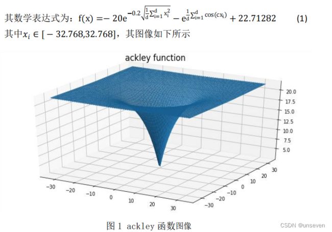
(1)ackley函数
ackley函数由指数函数加上放大的余弦函数所得的连续性函数,余弦波进行调制以形成波峰或波谷,它的特点是外部区域几乎平坦,中心有一个大孔。该函数有可能使优化算法,尤其是爬山算法,陷入其众多局部最小值之一,十分考验算法的寻优能力。
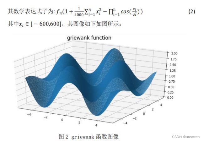
(2)griewank 函数
Griewank 函数是一个典型的多峰函数,全局最小值是唯一,位于原点,存 在大量局部极小值,这些最小值是有规律分布的,其复杂结构容易使优化算法陷 入局部最优解。
(3)rastrigin 函数
Rastrigin 函数是一个非凸、具有多个局部极小值的多峰函数,Rastrigin 函数因搜索空间大,存在大量局部极小值,求其全局最小值是一个相当棘手的问 题, Rastrigin 函数是高度多模态的,但最小值的位置是规则分布的。

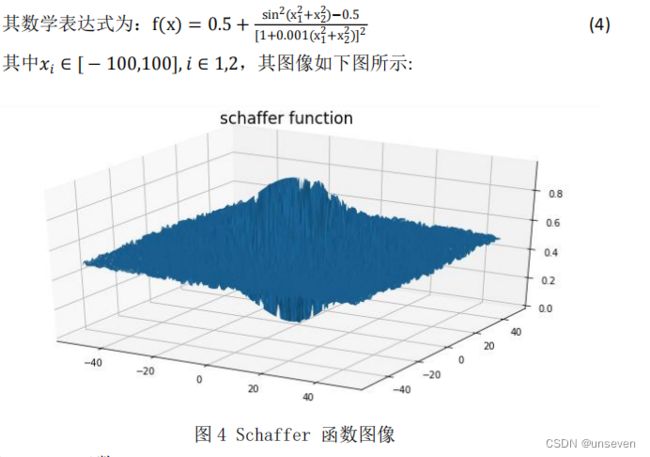
(4)schaffer 函数
Schaffer 函数是一个二维的多峰复杂函数,在其收敛范围内存在无数个极小 值点,只有一个全局最小值,在x1 = x2 = 0 处取得全局最小值,该函数因其强 烈振荡性质及其全局最优点被无数局部最优点所包围的特性使得一般算法很难 找到其全局最优点。
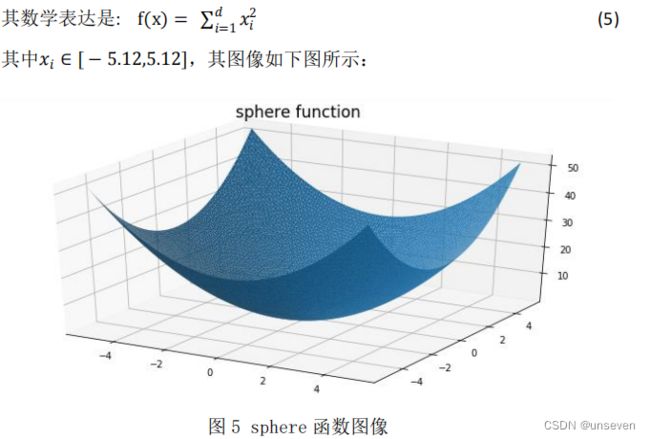
(5)sphere 函数
Sphere 函数是一个简单的单峰函数,只存在全局最优解,不存在局部最优解, 因此利用该函数可以较好的测试出优化算法的收敛速度。
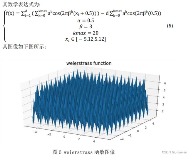
(6)weierstrass 函数
weierstrass 函数是第一个被发现的处处连续而处处不可导的函数,放大曲线 并不会显示它越来越接近直线。而是在任意两点之间,无论多近,函数都不会单 调。说明了所谓的“病态”函数的存在性,改变了当时数学家对连续函数的看法。
(7)six_hump_camel_back 函数
six_hump_camel_back 函数有六个局部最大值,其中两个是全局最大值.

(8)Modified_rastrigin 函数
简化版的 rastrigin 函数,其数学表达式如下:

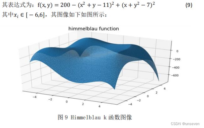
(9)himmelblau 函数
在数学优化中,Himmelblau 函数是一个多模态函数,用于测试优化算法的 性能
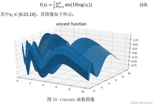
(10)vincent 函数
这是一个多模态最小化问题,定义如下:
二、 算法简介
(1)粒子群算法
粒子群算法要求每个个体在进化的过程中维护两个向量,就是速度向量 v i = [ v 1 i , v 2 i , . . . , v D i ] v_i= [v {1 \atop i}, v{2 \atop i}, . . . , v{D \atop i}] vi=[vi1,vi2,...,viD]和位置向量 x i = [ x 1 i , x 2 i , . . . , x D i ] x_i= [x{1 \atop i}, x{2 \atop i}, . . . , x{D \atop i}] xi=[xi1,xi2,...,xiD],其中 i 表示粒子的编号,D 是求解 问题的维度。粒子的速度决定的其运动的方向和速率,而位置则体现了粒子所代 表的解在解空间的位置,这也是评估这个解的质量的基础。算法要求每个粒子各 自维护一个自身的历史最优位置(PBset),如果粒子到达了某个至适应值更好 的位置,则将该位置记录到粒子的历史最优向量中,如果粒子能够不断的找到更 优的位置的话,该=向量也会不停的更新;群体还需要维护一个全局最优向量 (GBest),代表所有粒子的 PBest 中最优的那一个,这个全局最优向量起到了 引导粒子向全局最优收敛的作用.
粒子群算法求解过程如下:
- 先初始化所有粒子的速度和位置,并将 PBest 设为当前位置,而群体中 最优的 PBest 将作为 GBest。在本题中我们设置群体的粒子总数为 100。
- 在每一代的进化中,计算各个粒子的适应度函数值,即各个基准函数的 值。
- 如果粒子当前适应度比历史最优值要好,那么更新历史最优值。
- 如果粒子的适应度比全局最优值还要高,那么更新全局最优值。
- 每个粒子速度和位置更新方式为:

- 如果没达到结束条件,转到 2,否则输出 GBest 并结束
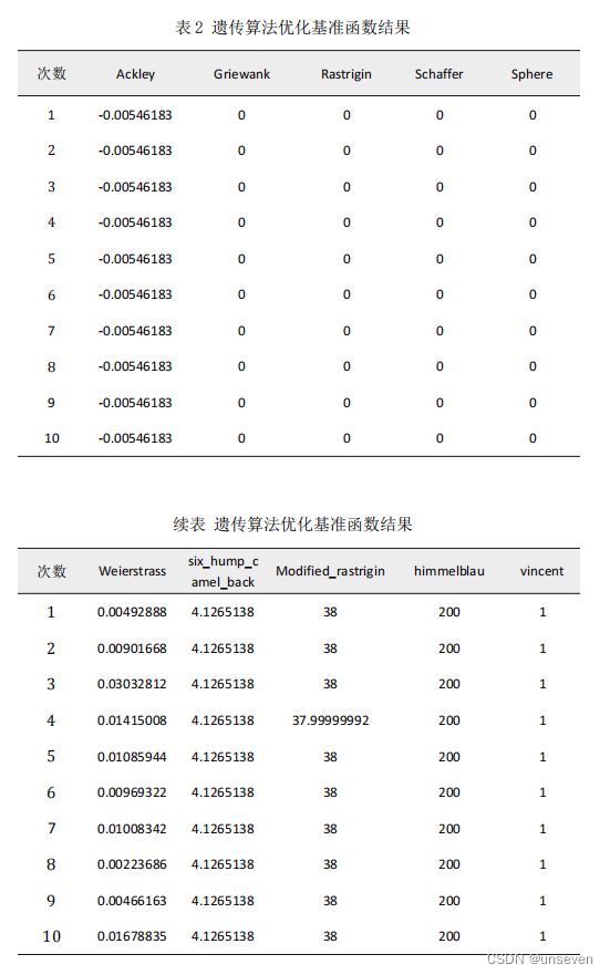
随机初始化种群,设置种群数量为 100,设置迭代次数为 100000 次,对每个 基准函数测试 10 次,其结果如下。

(2)遗传算法
生物的进化是一个不断往复的循环过程。在在每个循环过程中,自然环境 的恶劣、资源的短缺和天敌的侵害等因素,个体必须接受自然的选择。在选择过 程中,一部分对自然环境具有较高的适应能力的个体得以保存下来形成新的种 群。而另一部分个体则由于不适应自然环境而面临被淘汰的的危险。经过选择保 存下来的群体构成种群,种群的生物个体进行繁衍,保证了种群的发展。子代继 承了父代的部分特性,而且一般来说,子代要比父代具有更强的环境适应能力。 进化伴随着种群的变异,种群中的部分个体发生了基因变异,成为新的个体。这 样经过选择、交配和变异后的种群取代了原来的种群,进入下一个进化循环。
随机初始化种群,设置种群数量为 100,设置迭代次数为 100000 次,对每个 基准函数测试 10 次,其结果如下
(3)差分进化算法
从一个随机初始化的种群开始搜索,然后经过变异操作、交叉操作、选择操 作产生下一时刻的种群,该过程重复进行,直到满足停止条件。
交叉操作方式与遗传算法也大体相同,但在变异操作方面使用差分策略,即 利用种群中个体间的差分向量对个体进行扰动,实现个体变异。DE 的变异方式, 有效利用群体分布特性,提高算法的搜索能力,避免遗传算法中变异方式的不足。
变异操作有:
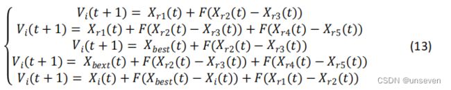
F 为 DE 的缩放因子,取值范围为[0,1]; x r 1 ( t ) x_{r1}(t) xr1(t)为从当前种群随机选择父代基 向量; x r 2 ( t ) − x r 3 ( t ) x_{r2}(t) − x_{r3}(t) xr2(t)−xr3(t)称为父代差分向量; r 1 , r 2 , r 3 r_1, r_2, r_3 r1,r2,r3是从随机选择的不同整数。
对第 g 代种群 v i ( g ) v_i(g) vi(g)及其变异的中间体 v i ( g + 1 ) v_i(g+ 1) vi(g+1)进行个体间的交叉操作,具体说明如下:
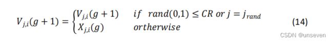
随机初始化种群,设置种群数量为 100,设置迭代次数为 100000 次, 对每个基准函数测试 10 次,其结果如下:

(4)分布估计算法
分布估计算法是一种基于种群的随机优化算法,它首先要生成一个初始种 群,然后通过建立概率模型和采样等操作使得种群得到不断地进化,直到达到结 束条件。其中建立概率模型和采样是分布估计算法地核心步骤,也是 EDA 算法 与 GA 算法的最大不同之处。由于分布估计算法没有“交叉”和“变异”操作, 因而通常不用基因来描述个体所包含的信息,取而代之的是变量。分布估计算法 通过分析较优群体包含的变量,构建符合这些变量分布的概率模型,然后基于该 概率模型再产生新的种群。因为概率模型是由种群中优势群体建立起来的,所以 基于该模型产生的新种群在整体质量上将优于原来的种群。由此推断,种群的整 体质量经过多次迭代后将不断得到提高,当前最优解一步一步逼近全局最优解。
基本流程为
- 初始群体,并对每一个个体进行估值;
- 根据个体估值,按照一定的选择策略从群体中选择的较优的个体;
- 根据选择的个体估计概率分布,建立相应的概率模型;
- 根据上一步估计得出的概率分布,采样产生新一代个体,并重新对每一 个新个体进行估值;
- 满足条件则停止,否则返回步骤2.
随机初始化种群,设置种群数量为 100,设置迭代次数为 100000 次,对每个 基准函数测试 10 次,其结果如下:

(5)蚁群算法
蚂蚁在寻找食物时,会在其经过的路径上释放一种信息素,并能够感知其他 蚂蚁释放的信息素。信息素浓度的大小表示路径的远近,浓度越高,表明对应的 路径距离越短。通常,蚂蚁会以较大的概率优先选择信息素浓度较高的路径,并释放一定量的信息素,这样就形成一个正反馈。最终,蚂蚁能够找到一条从巢穴 到食物源的最佳路径,即最短距离。同时,生物学家还发现,路径上的信息素浓 度会随着时间的推移而逐渐衰减。
- 首先初始化蚂蚁个数m、最大迭代次数 iter_max、信息发挥因子 Rho、转 移概率常熟 P 和搜索步长 step。
- 随机产生蚂蚁初始位置,根据适应度函数计算适应值 Tau,计算状态转移 概率,其公式如下

其中 max(Tau)表示信息素的最大值,Tau(i)表示蚂蚁 i 的信息素,P(iter,i) 表示第 iter 次迭代蚂蚁的转移概率值。 - 进行位置更新,当状态转移概率小于转哟概率常数时,进行局部搜素,其 搜索公式为

new 为待移动的位置,old 为蚂蚁当前的位置,r1为[-1.1]的随机数,step 为 局部搜索步长。
当状态转移概率大于状态转移常数时,则进行全局搜索,其公式为:
其中 r 2 r_2 r2为[-0.5,0.5]的随机数,range 为自变量的大小空间。 - 计算新的蚂蚁位置的适应值,判断蚂蚁是否移动,更新信息素,信息素的 更新公式为:

其中 Rho 为信息发挥因子,Tau 为信息素,f 为目标函数值。 - 判断是否满足终止条件,若满足,则结束搜索过程,输出最优值;若不满 足,则继续进行迭代。
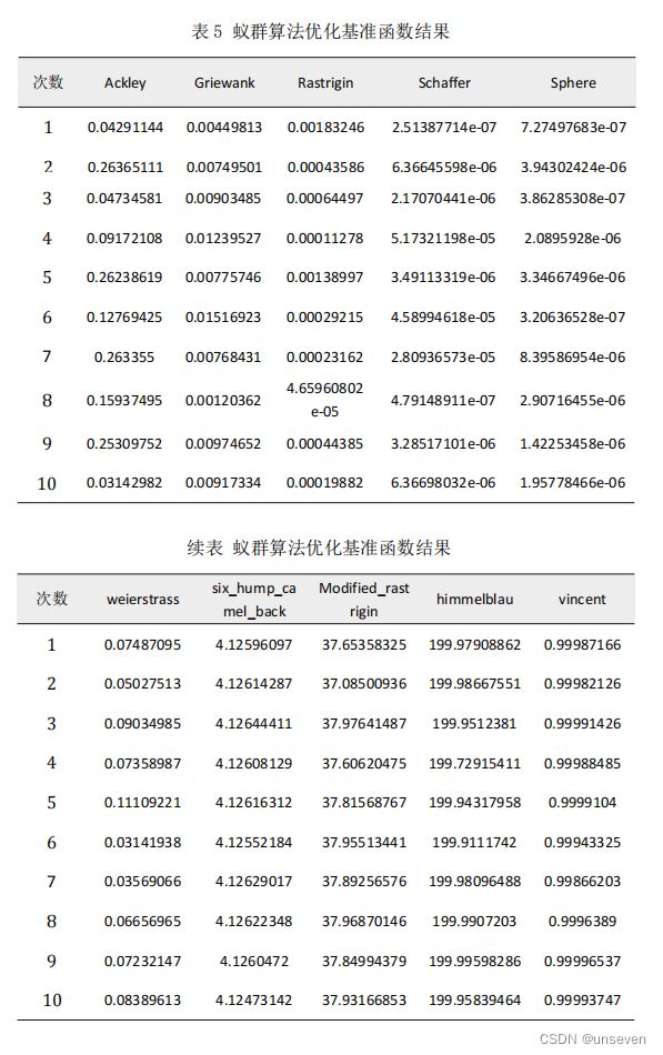
随机初始化种群,设置种群数量为 100,设置迭代次数为 100000 次,对每个 基准函数测试 10 次,其结果如下:
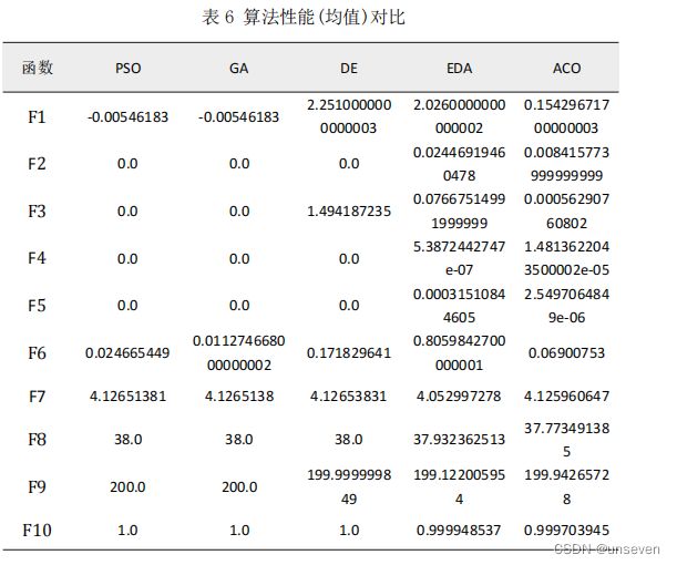
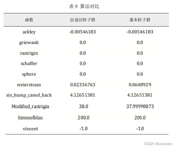
三、 算法性能对比
将各个算法独立运行 10 次的结果进行统计,比较其均值和方差,得到结果 如下表所示:

四、拓展题一
4.1 数据集处理
选择数字识别数据集作为本部分数据集,每一张图片为 28283 的 3 通道图 片,如下所示:
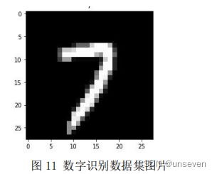
将其灰度化,并扁平化为一维数组,那么每一张图片将转化为 1*784 的特征, 最后再加上其标签。 将 60000 张图片进行同样处理,并将其存储为 csv 文件,将其打乱,选出 2000 个作为要优化的数据集。
4.2 特征选择
先建立 KNN 的分类模型,设定参数 k 值为 11,将选择的特征传入模型进行 准确率的求解,将 1-准确率最作为要优化的目标,特征选择的目的是使得错误率 最小,然后利用 PSO 和 DE 算法分别进行特征选择。
PSO 算法进行特征选择的的流程如下:
- 初始化速度。最大速度各个维度值全为 1,最小速度各个维度值全为 0, 速度初始化为最大速度和最小速度间的一个随机数。
- 将种群位置转化为二进制,并得到适应值。大于等于 0.5 的值全部替换为 1,否则替换为 0,为 1 则代表当前维度对应的特征应该被选择,为 0 则将这一 维特征淘汰,将处理好的数据集传入机器学习模型进行预测,将错误率作为适应 值返回。
- 更新种群的全局最优解以及个体的历史最优解。
- 更新速度和个体。根据全局最优解和历史最优解更新个体的速度,并进行 边界检查,个体加上速度移动到新的位置,然后对位置进行边界检查。
- 如果到了终止条件则停止,否则转入步骤 3。
DE 算法进行特征选择的流程如下:
- 初始化速度。最大速度各个维度值全为 1,最小速度各个维度值全为 0, 速度初始化为最大速度和最小速度间的一个随机数。
- 将种群位置转化为二进制,并得到适应值。大于等于 0.5 的值全部替换为 1,否则替换为 0,为 1 则代表当前维度对应的特征应该被选择,为 0 则将这一 维特征淘汰,将处理好的数据集传入机器学习模型进行预测,将错误率作为适应值返回.
- 更新种群的全局最优解以及全局最优值。
- 随机选择三个个体对当前个体进行差分进化,并进行边界检查。
- 进行交叉操作。如果到了设定的概率则对其进行交叉操作,否则保持原个 体不变,然后进行边界检查。由此得到新的种群。
- 如果新种群的个体适应值更好,则替换原有个体,否则保持原个体不变。
- 如果达到终止条件则停止进化,否则转入步骤 3。
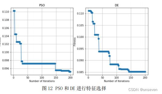
在 784 个特征里,PSO 最后选择了 419 维特征,模型的准确率达到了 89.83%, DE 选择 366 维特征,最后的准确率维 91%。
五、 拓展题 3
在这部分需要设计一个参数自适应的粒子群算法。那么粒子群主要有 3 个重要的参数,分别是惯性参数、全局学习参数以及局部学习参数。
如果 w 设为定值,那么随着迭代次数的增加导致问题求解的细节发生改变, 在整体求解的过程中存在不少缺陷,以求最小值为例,当适应值小时,说明距离 最优解越近,此时应该注重局部搜索,而当适应值大时,说明离最优解很远,应 该注重全局搜索。
引入变动的惯性权重,以适应动态问题的求解,故采用以下方式更新 w:
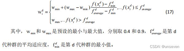
利用这一思想同样可以对学习因子进行更新,以求解最小值为例,随着迭代 次数的增加,适应度越来越小,即越来越接近全局最优值,此时应该更加重视局 部搜索。随着迭代次数的增加,局部学习参数应该增大,而全局学习参数应该减 小。其更新公式如下所示:

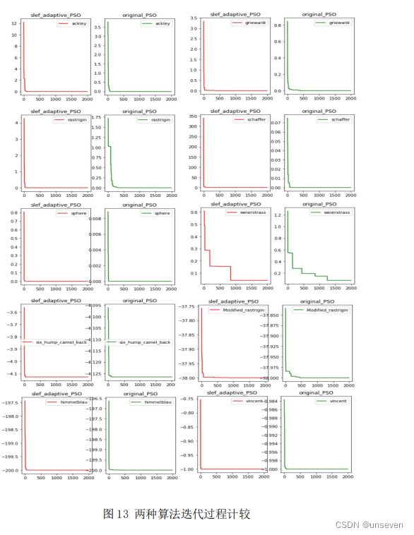
将自适应粒子群优化以上 10 个基准函数,并与基本粒子群算法进行比较(设 定随机数种子,使二者种群初始化相同),结果如下:
自适应的粒子群在同样的起始位置寻优能力略强于基本粒子群算法。
自适应粒子群算法和基本粒子群算法各个基准函数的迭代过程比较结果如下:
参考文献
[1] 张鑫礼. 多目标粒子群算法原理及其应用研究[D]. 内蒙古科技大学, 2015.
[2] 胡康. 一种改进粒子群算法及其应用[D]. 华北电力大学, 2019.
[3] 阎帅, 刘子旗, 刘昊城,等. 粒子群算法研究与进展[J]. 现代工业经济和 信息化, 2019, 9(03):19-20.
[4] 由睿鹏.计算机网络优化设计中遗传算法的原理及应用[J].电子技术与软件 工程,2020(20):14-15.
[5] [1]吕梦迪.遗传算法及其简单应用[J].大众标准化,2020(02):64-65.
[6] 贾 时 . 粒 子 群 与 差 分 进 化 混 合 算 法 的 研 究 及 应 用 [D]. 天 津 工 业 大学,2021.DOI:10.27357/d.cnki.gtgyu.2021.000233.
[7] 程吉祥. 自主差分进化算法设计及应用[D].西南交通大学,2015.
[8] 高尚,刘勇.基于分布估计算法的多目标优化[J].软件,2017,38(12):25-28.
[9] 董兵. 分布估计算法中差分采样策略的研究[D].华东师范大学,2017.
[10] 杨锐锐,王颖.蚁群算法的基本原理及参数设置研究[J].南方农 机,2018,49(13):38-39.
[11] 代婷婷,朱桂玲,胡晓飞.改进蚁群算法及其应用[J].洛阳理工学院学报 (自然科学版),2021,31(03):80-84.
[12] 王 欢 欢 . 基 于 蝙 蝠 和 粒 子 群 算 法 的 特 征 选 择 [D]. 西 北 师 范 大 学,2021.DOI:10.27410/d.cnki.gxbfu.2021.001829.
[13] 李炜,巢秀琴.改进的粒子群算法优化的特征选择方法[J].计算机科学与 探索,2019,13(06):990-1004.
[14] 王雪. 基于差分进化算法的特征选择方法研究[D].哈尔滨工程大 学,2020.DOI:10.27060/d.cnki.ghbcu.2020.002061.
[15] Abed-Alguni B H , Paul D , Hammad R . Improved Salp swarm algorithm for solving single-objective continuous optimization problems[J]. 2022.
[16] Best Vehicles Flow Traffic Light Controller Module Based on Particle Swarm Optimization (PSO)[J]. American Journal of Intelligent Systems,2018,8(1).
[17] [1]Liu Hao,Zhang Xue-Wei,Tu Liang-Ping. A Modified Particle Swarm Optimization Using Adaptive Strategy[J]. Expert Systems with Applications,2020,152(prepublish). [18] Sushanta Kumar Panigrahi,Amaresh Sahu,Sabyasachi Pattnaik. Structure Optimization Using Adaptive Particle Swarm Optimization[J]. Procedia Computer Science,2015,48©.
代码
1. 基准函数
###  benchmarks  基准测试函数集
import numpy as np
import matplotlib.pyplot as plt

class benchmarks():

    def ackley(x:np.ndarray,d=2)->np.ndarray :
        '''
        1
        由指数函数加上放大的余弦函数所得的连续性函数,余弦波进行调制以形成波峰或波谷,
        从而使函数图形表面波动,由于Ackley函数的独特性,
        导致Ackley函数在寻找全局最优解过程中不可避免地陷入局部最优解的陷阱
        x : [-32,768,32.768]
        '''
        fit = -20*np.e**( -0.2 * np.sqrt(  np.sum(x**2,axis=1) / d )  ) - np.e**(np.sum(np.cos(2*np.pi*x) , axis=1) / d ) + 22.71282
        return fit

    def griewank(x:np.ndarray,d=2):
        '''
        2
        Griewank函数是一个典型的多峰函数,全局最小值是唯一,位于原点,
        存在大量局部极小值,其复杂结构容易使优化算法陷入局部最优解。
        xi∈[−600,600]
        '''
        a1 = []
        for i in range(len(x)):
            a2 = []
            for j in range(len(x[i])):
                a2.append(x[i,j]/((j+1)**0.5))
            a1.append(a2)
        a1 = np.array(a1)
        fit = 1 + 1/4000*np.sum(x**2,axis=1)  - np.cumproduct(np.cos(a1),axis=1)[:,-1]
        return fit

    def rastrigin(x:np.ndarray,d=2)->np.ndarray:
        '''
        3
        Rastrigin函数是一个非凸、具有多个局部极小值的多峰函数,
        Rastrigin函数因搜索空间大,存在大量局部极小值,求其全局最小值是一个相当棘手的问题,
        Rastrigin函数是高度多模态的,但最小值的位置是规则分布的。
        xi∈[−5.12,5.12]
        '''
        fit = 10*d + np.sum( x**2 - 10*np.cos(2*np.pi*x) ,axis=1 )
        return fit

    def schaffer(x:np.ndarray,d=2)->np.ndarray:
        '''
        4
        Schaffer函数是一个二维的多峰复杂函数,在其收敛范围内存在无数个极小值点,
        只有一个全局最小值,在 x1=x2=0 处取得全局最小值
        该函数因其强烈振荡性质及其全局最优点被无数局部最优点所包围的特性使得一般算法很难找到其全局最优点
        xi∈[−100,100]
        '''
        fit = []
        for i in range(len(x)):
            f = 0.5 + (np.sin(x[i,0]**2 - x[i,1]**2) **2 -0.5)  / (1 + 0.001*(x[i,0]**2 + x[i,1]**2 )  )**2
            fit.append(f)
        return np.array(fit)

    def sphere(x:np.ndarray,d=2)->np.ndarray:
        '''
        5
        Sphere函数是一个简单的单峰函数,只存在全局最优解,
        不存在局部最优解,因此可利用该函数可以较好的测试出优化算法的收敛速度。
        xi∈[−50,50]
        '''
        fit = np.sum(x**2,axis=1)
        return fit

    def weierstrass(x:np.ndarray,d=2)->np.ndarray:
        '''
        6
        是第一个被发现的处处连续而处处不可导的函数,
        说明了所谓的“病态”函数的存在性,改变了当时数学家对连续函数的看法
        α=0.5,β=3,kmax=20
        '''
        a,b,K = 0.5,3,20
        fit = []
        for j in range(len(x)):
            t1 = 0
            for i in range(d):
                for k in range(K):
                    t1 += a**k * np.cos(2*np.pi*(b**k)*( x[j,i]+0.5))
            t2 = 0
            for k in range(K):
                t2 += a**k * np.cos( 2*np.pi * (b**k)*0.5 )
            t2 = t2*d
            fit.append(t1-t2)
        return np.array(fit)

    def six_hump_camel_back(x:np.ndarray,d=2)->np.ndarray:
        '''
        7
        六峰值驼背函数
        xϵ[−1.9,1.9]y ϵ [ − 1.1 , 1.1 ]
        '''
        fit = []
        for i in range(len(x)):
            f = -4* (  (4 - 2.1*x[i,0]**2 + (x[i,0]**4)/3 )*x[i,0]**2  + x[i,0]*x[i,1] + (4*(x[i,1]**2) - 4)*x[i,1]**2                                  )
            fit.append(f)
        return -np.array(fit)

    def Modified_rastrigin(x:np.ndarray,d=2)->np.ndarray:
        '''
        8
        简化版的rastrigin函数
        xiϵ[0,1]
        '''
        fit = -np.sum(10 + 9*np.cos(2*np.pi*x),axis=1)
        return fit

    def himmelblau(x:np.ndarray,d=2)->np.ndarray:
        '''
        9
        Himmelblau函数是用来测试后话算法的常用阳历函数之一,它包含了两个自变量x和y
        x ϵ [ − 6 , 6 ]
        '''
        fit = []
        for i in range(len(x)):
            f = 200 - (x[i,0]**2 + x[i,1] - 11)**2  -(x[i,0] + x[i,1]**2 - 7)**2
            fit.append(f)
        return -np.array(fit)

    def vincent(x:np.ndarray,d=2)->np.ndarray:
        '''
        10
        '''
        fit = 1/d * np.sum( np.sin(10*np.log10(x)),axis=1  )
        return fit


def tanh (x:np.ndarray)->np.ndarray:
    return (np.e**x-np.e**(-x))/(np.e**x+np.e**(-1))*100
def log(x):
    f = []
    for each in x:
        if each > 1:
            f.append(np.log(each))
        elif -1<each<1:
            f.append(0)
        else:
            f.append(-np.log(-each))
    return f
2. 遗传算法
# GA算法   遗传算法
import numpy as np
import matplotlib.pylab as plt


def GA(lb,ub,popsize=100,dim=2,maxIter=1000):
    def cross(pop):
        for i in range(len(pop)):
            probability = np.random.randint(1,101)
            if probability<=10:  ##设定发生交叉的概率为0.1
                slice1,slice2 = np.random.randint(0,len(pop[0])),np.random.randint(0,len(pop[0]))
                temp,temp1 = max(slice1,slice2),min(slice1,slice2)
                slice1,slice2 = temp1,temp
                temp = pop[i][slice1:slice2]
                index = np.random.randint(0,len(pop))
                pop[i][slice1:slice2] = pop[index][slice1:slice2]
                pop[index][slice1:slice2] = temp
        return pop


    # 初始化过程
    pop = np.random.uniform(lb,ub,(popsize,dim))  # generate population
    individualBest = pop.copy() # location and the individual best
    velocity = pop.copy() # velocity of every particle


    fit = benchmarks.vincent(pop) # 适应值评估    ## 替换为基准函数
    globalBest = pop[0] # 指定全局最优解

    # 初始化过程结束,进入迭代过程
    fitBest = []  # 用列表存储每一代的最优值
    omiga,c1,c2 = 0.7,1.4,1.4 # 对应于w,c1,c2的参数表
    for i in range(maxIter):
        # if i % 2000 == 0:
        #     print("gen:{}, globalBestFit:{}".format(i, globalBest ))
        r1 = np.random.random(); r2 = np.random.random() # 生成两个随机数
        # 更新速度和位置
        velocity = velocity * omiga + r1*c1*(globalBest - pop) + r2*c2*(individualBest - pop) #
        pop += velocity

        pop = cross(pop) ##  将更新后的种群进行交叉操作
        #合法性检查
        beyondLb = np.random.uniform(lb,ub);  beyondUb = np.random.uniform(lb,ub)  # 越界处理机制
        temp = np.where(pop<lb,beyondLb,pop)
        pop = np.where(temp>ub,beyondUb,temp)

        # #评价
        fitCurrent = benchmarks.vincent(pop) ## 替换为基准函数

        #更新历史最优解和个体最优解
        ind = fitCurrent<fit   ##  最大最小值更改
        individualBest = np.vstack((pop[ind],individualBest[~ind])).copy() # 更新个体最优历史
        fit = np.hstack((fitCurrent[ind],fit[~ind])).copy() # 更新适应值
        globalBest = pop[np.argmin(fitCurrent)] #群体最优值
        fitBest.append(np.min(fit))  # 记录每一代最优值。
    return fitBest

fitBest = GA(lb=0.25,ub=10,popsize=10,maxIter=1000)
fitBest = np.array(fitBest)
# print(fitBest)
fitBest1 = tanh(fitBest)
# print(fitBest1)
print(fitBest[-5:]) # 输出最后五个值
# 汇出函数图像。为了便于观察,取适应值的对数。
plt.plot(fitBest1,color='g')
# plt.plot(fitBest,color='r')
plt.title('GA')
plt.show()

# plt.plot(fitBest1,color='g')
plt.plot(fitBest,color='r')
plt.title('GA')

plt.show()
3. 粒子群算法
import numpy as np
import matplotlib.pyplot as plt

class PSO:
    def __init__(self,lb=-10,ub=10,popsize=100,dim=2):
        self.lb = lb
        self.ub = ub
        self.popsize = popsize
        self.dim = dim
        self.pop = np.random.uniform(lb, ub, (popsize, dim))  # generate population
        self.individualBest = self.pop.copy()  # location and the individual best
        self.velocity = self.pop.copy()  # velocity of every particle
        self.fit = benchmarks.vincent(self.pop) ## 替换为基准函数
        self.globalBest = self.pop[0]  # 指定全局最优解


    def sovle(self,maxIter =1000):
        fitBest = []  # 用列表存储每一代的最优值
        omiga, c1, c2 = 0.7, 1.4, 1.4  # 对应于w,c1,c2的参数表
        for i in range(maxIter):
            # if i % 50 == 0:
            #     print("gen:{}, globalBestFit:{}".format(i, self.globalBest ))
            r1 = np.random.random()
            r2 = np.random.random()  # 生成两个随机数
            # 更新速度和位置
            self.velocity = self.velocity * omiga + r1 * c1 * (self.globalBest - self.pop) + r2 * c2 * (self.individualBest - self.pop)  #
            self.pop += self.velocity

            # 合法性检查
            beyondLb = np.random.uniform(self.lb, self.ub)
            beyondUb = np.random.uniform(self.lb, self.ub)  # 越界处理机制
            temp = np.where(self.pop < self.lb, beyondLb, self.pop)
            self.pop = np.where(temp > self.ub, beyondUb, temp)

            # #评价
            fitCurrent = benchmarks.vincent(self.pop) ## 替换为基准函数
            # 更新历史最优解和个体最优解
            ind = fitCurrent < self.fit ## 最大最小更改
            self.individualBest = np.vstack((self.pop[ind], self.individualBest[~ind])).copy()  # 更新个体最优历史
            self.fit = np.hstack((fitCurrent[ind], self.fit[~ind])).copy()  # 更新适应值
            self.globalBest = self.pop[np.argmin(fitCurrent)]  # 群体最优值
            fitBest.append(np.min(self.fit))  # 记录每一代最优值。
        return fitBest
        # print(fitBest[-5:])  # 输出最后五个值
        # # 汇出函数图像。为了便于观察,取适应值的对数。
        # plt.plot(np.log(fitBest))
        # plt.show()


pso = PSO(lb=0.25,ub=10,popsize=10)
fitBest = pso.sovle(1000)
fitBest = np.array(fitBest)
# print(fitBest)
fitBest1 = tanh(fitBest)
# print(fitBest1)
print(fitBest[-5:]) # 输出最后五个值
# 汇出函数图像。为了便于观察,取适应值的对数。
plt.plot(fitBest1,color='g')
# plt.plot(fitBest,color='r')
plt.title('PSO')
plt.show()
4. 差分进化
import numpy as np
import matplotlib.pyplot as plt


#%% functions

def  DE(lb=-10,ub =10,ps=100,dim = 2,maxiter  = 1000):
    # mutation 变异
    def mutation(xpop,F,K,ind):
        # 共5种变异方式,写出一个作为样例,请写其他方式。
        m,n = xpop.shape
        ps = xpop.shape[0]
        serial = np.arange(0,ps)
        ind1 = np.random.permutation(serial) ## 对序列做一个变换
        ind2 = np.random.permutation(serial)
        ind3 = np.random.permutation(serial)
        ind4 = np.random.permutation(serial)
        ind5 = np.random.permutation(serial)
        if ind == 1 :
            mupop = xpop[ind1] + F*(xpop[ind2] - xpop[ind3])
        elif ind == 2:
            mupop = xpop[ind1] + F*(xpop[ind2] - xpop[ind3]) + F*(xpop[ind4] - xpop[ind5])
        elif ind == 3:
            mupop = bestfit[-1] + F*(xpop[ind2] - xpop[ind3])
        elif ind == 4:
            mupop = bestfit[-1] + F*(xpop[ind2] - xpop[ind3]) + F*(xpop[ind4] - xpop[ind5])
        elif ind == 5:
            mupop = xpop + F*( bestfit[-1]-xpop ) + F*( xpop[ind1] - xpop[ind2] )

        return mupop

    # 交叉操作
    def crossover(xpop,mupop,cr):
        ps,dim = mupop.shape
        flag = cr < np.random.rand(ps,dim)  ##  得到一个0,1矩阵
        # jrand = np.random.randint(0,dim,ps)
        # flag[:,jrand] = 1
        crpop =  mupop*flag + xpop*(1-flag)
        return crpop

    # boundary check
    def boundcheck(crpop,lb,ub):
        temp = np.random.uniform(lb,ub,crpop.shape)
        u = crpop > lb
        crpop = crpop * u + temp * (1-u)
        v = crpop < ub
        crpop =  crpop * v + temp * (1-v)
        return crpop

    def selection(pop,fit,crpop,cfit):
        ps,dim = pop.shape
        u = fit < cfit  #convert list to a numpy   ## 最大最小值更改
        fit = fit*u + cfit*(1-u)
        mu = np.repeat(u,dim).reshape(-1,dim)
        pop = pop*mu + crpop*(1-mu)

        return pop,fit


    F,K = 0.3,0.5
    cr = 0.8

    # 初始化群体
    # pop = np.random.uniform(lb,ub,[ps,dim])
    pop = np.random.uniform(lb,ub,[ps,dim])  ## 生成初始种群
    bestfit = [min(benchmarks.vincent(pop))]  ## 替换为基准函数
    pop = np.random.uniform(lb,ub,[ps,dim])  ## 生成初始种群
    # print(len(pop) )
    for i in range(maxiter):
        xpop = pop.copy()
        # fit = evaluate(prob,xpop)
        # print((fit))
        fit = benchmarks.vincent(xpop)      ## 替换为基准函数
        # print(len(fit))
        mupop = mutation(xpop, F, K, ind=3)
        crpop = crossover(xpop, mupop, cr)
        newpop = boundcheck(crpop, lb, ub)
        # cfit = evaluate(prob, newpop)
        cfit = benchmarks.vincent( newpop)       ## 替换为基准函数
        pop,fit = selection(xpop, fit, newpop, cfit)
        bestfit.append(min(fit))
        # if ~(i % 100):
        #     print("problem = {} gen={}  bestfit={}".format(prob,i,bestfit[-1]))
    return bestfit

fitBest = DE(lb=0.25,ub=10,ps=100,maxiter=1000)
fitBest = np.array(fitBest)
fitBest1 = tanh(fitBest)
print(fitBest[-5:]) # 输出最后五个值
plt.plot(fitBest1,color='g')
plt.title('DE')
plt.show()
5. 分布估计算法
def  EDA(lb=-10,ub =10,ps=100,dim = 2,maxiter  = 1000):
    # 初始化群体
    # pop = np.random.uniform(lb,ub,[ps,dim])
    pop = np.random.uniform(lb,ub,[ps,dim])  ## 生成初始种群
    u = np.mean(pop)  ## u为pop的均值
    v = np.var(pop)   ## v为pop的方差
    # print(len(pop) )
    x1 = pop[:,0]
    x2 = pop[:,1]
    u1=np.mean(x1)  ### xi的均值
    u2=np.mean(x2)
    v1=np.var(x1)   ## xi的方差
    v2=np.var(x2)
    a=0.1   #learn rate
    K=5 #选取的最优的样本的个数
    bestfit = []
    for i in range(maxiter):
        fit = benchmarks.vincent(pop).tolist()   ## 替换为基准函数
        d = sorted(fit,reverse=False)  ##  最大最小值更改,false为求最小值
        # print(d)
        bestfit.append(min(fit))
        x1 = pop[:,0].tolist()
        x2 = pop[:,1].tolist()
        first_max=fit.index(d[0])   ##  选出最大值适应值对应的下标
        second_max=fit.index(d[1])  ## 第二大的适应值对应的下标
        min_=fit.index(d[-1])       ## 最小适应值对应的下标
        u1=(1-a)*u1+a*(x1[first_max]+x1[second_max]-x1[min_])  ## 更新ui
        u2=(1-a)*u1+a*(x2[first_max]+x2[second_max]-x2[min_])
        aver1=(x1[fit.index(d[0])]+x1[fit.index(d[1])]+x1[fit.index(d[2])]+x1[fit.index(d[3])]+x1[fit.index(d[4])])/K  ## 优势种群的均值
        aver2=(x2[fit.index(d[0])]+x2[fit.index(d[1])]+x2[fit.index(d[2])]+x2[fit.index(d[3])]+x2[fit.index(d[4])])/K
        total1=abs(x1[fit.index(d[0])]-aver1)+abs(x1[fit.index(d[1])]-aver1)+abs(x1[fit.index(d[2])]-aver1) + abs(x1[fit.index(d[3])]-aver1)+ abs(x1[fit.index(d[4])]-aver1)
        total1=round(total1,2)
        # print("total1",total1)
        total2=abs(x2[fit.index(d[0])]-aver2) + abs(x2[fit.index(d[1])]-aver2) + abs(x2[fit.index(d[2])]-aver2) + abs(x2[fit.index(d[3])]-aver2) + abs(x2[fit.index(d[4])]-aver2)
        total2=round(total2,2)
        # print("total2",total2)
        v1=abs((1-a)*v1+a*(total1/K)**0.5)
        v2=abs((1-a)*v2+a*(total2/K)**0.5)
        x1=np.random.normal(u1,v1,ps)
        x2=np.random.normal(u2,v2,ps)
        tmp = []
        for i in range(len(x1)):
            t = [x1[i],x2[i]]
            tmp.append(t)
        pop = np.array(tmp)
    return bestfit

fitBest = EDA(lb=0.25,ub=10,ps=100,maxiter=1000)
fitBest = np.array(fitBest)
fitBest1 = tanh(fitBest)

print(fitBest[-5:]) # 输出最后五个值
plt.plot(fitBest,color='g')
plt.title('EDA')
plt.show()
6. 蚁群算法
def AG(lb=-10,ub =10,ps=100,dim = 2,maxiter  = 1000):
    ## 边界处理
    def boundcheck(crpop,lb,ub):
        temp = np.random.uniform(lb,ub,crpop.shape)
        u = crpop > lb
        crpop = crpop * u + temp * (1-u)
        v = crpop < ub
        crpop =  crpop * v + temp * (1-v)
        return crpop
    ## 初始化参数
    m = ps                    # 蚂蚁数量
    iter_max = maxiter              # 最大迭代次数
    Rho = 0.9                  # 信息素挥发因子
    P0 = 0.2                   # 转移概率常数
    step = 0.05                # 局部搜索步长
    Tau = np.zeros((m, 1))          # 信息素矩阵
    P = np.zeros((iter_max, m))     # 转移概率矩阵
    bestfit = []                    # 历代最优值
    ant = np.random.uniform(lb,ub,[ps,dim])  ## 生成初始蚁群
    Tau = benchmarks.vincent(ant)             ## 信息素矩阵,即适应值函数   ## 替换为基准函数
    for iterr in range(1,maxiter):
        lam = 1/iterr
        Tau_best,BestIndex = max(Tau),Tau.argmax   ## 最大适应值及其下标
        P = (Tau_best - Tau)/Tau_best              ## 状态转移概率
        P1 = P<P0           ## 概率小于P0的部分用局部搜索
        P1 = P1.repeat(repeats=2).reshape(-1,2)  ## 0,1矩阵
        # print(P1)
        # print(ant)
        ant1 = ant +(2*np.random.rand(ps,2)-1)*step*lam
        ant1 = ant1*P1       ## 只保留概率小的部分
        # print(ant1)
        P2 = P>=P0     ## 概率大的部分用全局搜素
        P2 = P2.repeat(repeats=2).reshape(-1,2)  ## 0,1矩阵
        ant2 = ant + (ub-lb)*(np.random.rand(ps,2)-0.5)
        ant2 = ant2*P2       ## 只保留概率大的
        # print(ant2)
        xant = ant1 + ant2    ## 局部搜素和全局搜素汇总,构成一个新的蚁群
        xant = boundcheck(xant,lb,ub)  ## 检查是否越界
        xTau = benchmarks.vincent(xant)   ## 评价新的种群  ## 替换为基准函数
        ##  根据求最大值还是最小值改变符号
        P3 = xTau < Tau  ## 新蚁群中好的个体   ## 最大最小值更改
        P3 = P3.repeat(repeats=2).reshape(-1,2)  ## 0,1矩阵
        P4 = xTau >= Tau  ## 旧蚁群中好的个体    ##  最大最小值更改
        P4 = P4.repeat(repeats=2).reshape(-1,2)  ## 0,1矩阵
        # print(P3)
        # print(P4)
        ant = ant*P4 + xant*P3   ## 将新旧两代好的个体汇总才是真正的下一代蚁群
        fit = benchmarks.vincent(ant)    ## 替换为基准函数
        Tau = Tau*(1-Rho) + fit ## 更新信息素
        bestfit.append(min(fit))
    return bestfit


fitBest = AG(lb=0.25,ub=10,ps=100,maxiter=1000)
fitBest = np.array(fitBest)
fitBest1 = tanh(fitBest)

print(fitBest[-5:]) # 输出最后五个值
plt.plot(fitBest1,color='g')
plt.title('AG')
plt.show()
7. PSO特征选择
import numpy as np
from numpy.random import rand

## 初始化种群
def init_position(lb, ub, N, dim):
    X = np.zeros([N, dim], dtype='float')
    for i in range(N):
        for d in range(dim):
            X[i,d] = lb[0,d] + (ub[0,d] - lb[0,d]) * rand()
    return X

## 初始化速度
def init_velocity(lb, ub, N, dim):
    V    = np.zeros([N, dim], dtype='float')
    Vmax = np.zeros([1, dim], dtype='float')
    Vmin = np.zeros([1, dim], dtype='float')
    # Maximum & minimum velocity
    for d in range(dim):
        Vmax[0,d] = (ub[0,d] - lb[0,d]) / 2
        Vmin[0,d] = -Vmax[0,d]

    for i in range(N):
        for d in range(dim):
            V[i,d] = Vmin[0,d] + (Vmax[0,d] - Vmin[0,d]) * rand()

    return V, Vmax, Vmin

## 转化为二进制
def binary_conversion(X, thres, N, dim):
    Xbin = np.zeros([N, dim], dtype='int')
    for i in range(N):
        for d in range(dim):
            if X[i,d] > thres:
                Xbin[i,d] = 1
            else:
                Xbin[i,d] = 0

    return Xbin

## 边界检查
def boundary(x, lb, ub):
    if x < lb:
        x = lb
    if x > ub:
        x = ub

    return x


def jfs_pso(xtrain, ytrain, opts):
    # Parameters
    ub    = 1
    lb    = 0
    thres = 0.5
    w     = 0.9    # inertia weight
    c1    = 2      # acceleration factor
    c2    = 2      # acceleration factor

    N        = opts['N']
    max_iter = opts['T']
    if 'w' in opts:
        w    = opts['w']
    if 'c1' in opts:
        c1   = opts['c1']
    if 'c2' in opts:
        c2   = opts['c2']

    # Dimension
    dim = np.size(xtrain, 1)
    if np.size(lb) == 1:
        ub = ub * np.ones([1, dim], dtype='float')
        lb = lb * np.ones([1, dim], dtype='float')

    # 初始化种群和速度
    X             = init_position(lb, ub, N, dim)
    V, Vmax, Vmin = init_velocity(lb, ub, N, dim)

    # Pre
    fit   = np.zeros([N, 1], dtype='float')
    Xgb   = np.zeros([1, dim], dtype='float')
    fitG  = float('inf')
    Xpb   = np.zeros([N, dim], dtype='float')
    fitP  = float('inf') * np.ones([N, 1], dtype='float')
    curve = np.zeros([1, max_iter], dtype='float')
    t     = 0

    while t < max_iter:
        # Binary conversion
        Xbin = binary_conversion(X, thres, N, dim)

        # Fitness
        for i in range(N):
            fit[i,0] = Fun(xtrain, ytrain, Xbin[i,:], opts)
            if fit[i,0] < fitP[i,0]:
                Xpb[i,:]  = X[i,:]
                fitP[i,0] = fit[i,0]
            if fitP[i,0] < fitG:
                Xgb[0,:]  = Xpb[i,:]
                fitG      = fitP[i,0]

        # Store result
        curve[0,t] = fitG.copy()
        if t % 10 == 0:
            print("Iteration:", t + 1)
            print("Best (PSO):", curve[0,t])
        # print(len(sel_index))
        t += 1

        for i in range(N):
            for d in range(dim):
                # Update velocity
                r1     = rand()
                r2     = rand()
                V[i,d] = w * V[i,d] + c1 * r1 * (Xpb[i,d] - X[i,d]) + c2 * r2 * (Xgb[0,d] - X[i,d])
                # Boundary
                V[i,d] = boundary(V[i,d], Vmin[0,d], Vmax[0,d])
                # Update position
                X[i,d] = X[i,d] + V[i,d]
                # Boundary
                X[i,d] = boundary(X[i,d], lb[0,d], ub[0,d])


    # Best feature subset
    Gbin       = binary_conversion(Xgb, thres, 1, dim)
    Gbin       = Gbin.reshape(dim)
    pos        = np.asarray(range(0, dim))
    sel_index  = pos[Gbin == 1]
    num_feat   = len(sel_index)
    # Create dictionary
    pso_data = {'sf': sel_index, 'c': curve, 'nf': num_feat}

    return pso_data
8. DE特征选择
import numpy as np
from numpy.random import rand


def init_position(lb, ub, N, dim):
    X = np.zeros([N, dim], dtype='float')
    for i in range(N):
        for d in range(dim):
            X[i,d] = lb[0,d] + (ub[0,d] - lb[0,d]) * rand()

    return X


def binary_conversion(X, thres, N, dim):
    Xbin = np.zeros([N, dim], dtype='int')
    for i in range(N):
        for d in range(dim):
            if X[i,d] > thres:
                Xbin[i,d] = 1
            else:
                Xbin[i,d] = 0

    return Xbin


def boundary(x, lb, ub):
    if x < lb:
        x = lb
    if x > ub:
        x = ub

    return x


def jfs_de(xtrain, ytrain, opts):
    # Parameters
    ub    = 1
    lb    = 0
    thres = 0.5
    CR    = 0.9     # crossover rate
    F     = 0.5     # factor

    N        = opts['N']
    max_iter = opts['T']
    if 'CR' in opts:
        CR   = opts['CR']
    if 'F' in opts:
        F    = opts['F']

    # Dimension
    dim = np.size(xtrain, 1)
    if np.size(lb) == 1:
        ub = ub * np.ones([1, dim], dtype='float')
        lb = lb * np.ones([1, dim], dtype='float')

    # Initialize position
    X     = init_position(lb, ub, N, dim)

    # Binary conversion
    Xbin  = binary_conversion(X, thres, N, dim)

    # Fitness at first iteration
    fit   = np.zeros([N, 1], dtype='float')
    Xgb   = np.zeros([1, dim], dtype='float')
    fitG  = float('inf')

    for i in range(N):
        fit[i,0] = Fun(xtrain, ytrain, Xbin[i,:], opts)
        if fit[i,0] < fitG:
            Xgb[0,:] = X[i,:]
            fitG     = fit[i,0]

    # Pre
    curve = np.zeros([1, max_iter], dtype='float')
    t     = 0

    curve[0,t] = fitG.copy()
    print("Generation:", t + 1)
    print("Best (DE):", curve[0,t])
    t += 1

    while t < max_iter:
        V = np.zeros([N, dim], dtype='float')
        U = np.zeros([N, dim], dtype='float')

        for i in range(N):
            # Choose r1, r2, r3 randomly, but not equal to i
            RN = np.random.permutation(N)
            for j in range(N):
                if RN[j] == i:
                    RN = np.delete(RN, j)
                    break

            r1 = RN[0]
            r2 = RN[1]
            r3 = RN[2]
            # mutation (2)
            for d in range(dim):
                V[i,d] = X[r1,d] + F * (X[r2,d] - X[r3,d])
                # Boundary
                V[i,d] = boundary(V[i,d], lb[0,d], ub[0,d])

            # Random one dimension from 1 to dim
            index = np.random.randint(low = 0, high = dim)
            # crossover (3-4)
            for d in range(dim):
                if (rand() <= CR)  or  (d == index):
                    U[i,d] = V[i,d]
                else:
                    U[i,d] = X[i,d]

        # Binary conversion
        Ubin = binary_conversion(U, thres, N, dim)

        # Selection
        for i in range(N):
            fitU = Fun(xtrain, ytrain, Ubin[i,:], opts)
            if fitU <= fit[i,0]:
                X[i,:]   = U[i,:]
                fit[i,0] = fitU

            if fit[i,0] < fitG:
                Xgb[0,:] = X[i,:]
                fitG     = fit[i,0]


        # Store result
        curve[0,t] = fitG.copy()
        if t%10 == 0:
            print("Generation:", t + 1)
            print("Best (DE):", curve[0,t])
        t += 1


    # Best feature subset
    Gbin       = binary_conversion(Xgb, thres, 1, dim)
    Gbin       = Gbin.reshape(dim)
    pos        = np.asarray(range(0, dim))
    sel_index  = pos[Gbin == 1]
    num_feat   = len(sel_index)
    # Create dictionary
    de_data = {'sf': sel_index, 'c': curve, 'nf': num_feat}

    return de_data
9. 构建机器学习模型
import numpy as np
from sklearn.neighbors import KNeighborsClassifier
from sklearn.metrics import confusion_matrix,classification_report,precision_score

# error rate
def error_rate(xtrain, ytrain, x, opts):
    # parameters
    k     = opts['k']
    fold  = opts['fold']
    xt    = fold['xt']
    yt    = fold['yt']
    xv    = fold['xv']
    yv    = fold['yv']

    # Number of instances
    num_train = np.size(xt, 0)
    num_valid = np.size(xv, 0)
    # Define selected features
    xtrain  = xt[:, x == 1]
    ytrain  = yt.reshape(num_train)
    xvalid  = xv[:, x == 1]
    yvalid  = yv.reshape(num_valid)


    # Training
    # 若是回归问题,则使用回顾算法构建模型。
    mdl     = KNeighborsClassifier(n_neighbors = k)
    mdl.fit(xtrain, ytrain)
    # Prediction
    ypred   = mdl.predict(xvalid)
    # acc     = np.sum(yvalid == ypred) / num_valid
    acc = precision_score(yvalid,ypred,average='macro')
    error   = 1 - acc

    return error


# Error rate & Feature size
def Fun(xtrain, ytrain, x, opts):
    alpha    = 0.99
    beta     = 1 - alpha
    max_feat = len(x)
    # Number of selected features
    num_feat = np.sum(x == 1)
    # Solve if no feature selected
    if num_feat == 0:
        cost  = 1
    else:
        # Get error rate
        error = error_rate(xtrain, ytrain, x, opts)
        # Objective function
        cost  = alpha * error + beta * (num_feat / max_feat)

    return cost
10. 特征选择过程
import numpy as np
import pandas as pd
from sklearn.neighbors import KNeighborsClassifier
from sklearn.model_selection import train_test_split
import matplotlib.pyplot as plt


# load data
data  = pd.read_csv('test.csv')[:2000]
data  = data.values
feat  = np.asarray(data[:, 0:-1])
label = np.asarray(data[:, -1])

# split data into train & validation (70 -- 30)
xtrain, xtest, ytrain, ytest = train_test_split(feat, label, test_size=0.3, stratify=label)
fold = {'xt':xtrain, 'yt':ytrain, 'xv':xtest, 'yv':ytest}   ## 定义简写

# parameter
k    = 5     # k-value in KNN
N    = 10    # number of particles
T    = 200   # maximum number of iterations
opts = {'k':k, 'fold':fold, 'N':N, 'T':T}   ## 定义参数

# perform feature selection
fmdl = jfs_pso(feat, label, opts)  # 以数据字典的形式返回选择后的数据集  {'sf': sel_index, 'c': curve, 'nf': num_feat}
sf   = fmdl['sf']

# model with selected features
num_train = np.size(xtrain, 0)
num_valid = np.size(xtest, 0)
x_train   = xtrain[:, sf]
y_train   = ytrain.reshape(num_train)  # Solve bug
x_valid   = xtest[:, sf]
y_valid   = ytest.reshape(num_valid)  # Solve bug

mdl       = KNeighborsClassifier(n_neighbors = k)
mdl.fit(x_train, y_train)

# accuracy
y_pred    = mdl.predict(x_valid)
Acc       = np.sum(y_valid == y_pred)  / num_valid
print("Accuracy:", 100 * Acc)

# number of selected features
num_feat = fmdl['nf']
print("Feature Size:", num_feat)

# plot convergence
curve   = fmdl['c']
curve   = curve.reshape(np.size(curve,1))
x       = np.arange(0, opts['T'], 1.0) + 1.0


plt.figure(figsize=(10,5))
plt.subplot(1,2,1)
plt.plot(x, curve, 'o-')
plt.xlabel('Number of Iterations')
plt.ylabel('Fitness')
plt.title('PSO')
plt.grid()


# -----------      DE     -----------
# load data
data  = pd.read_csv('test.csv')[:2000]
data  = data.values
feat  = np.asarray(data[:, 0:-1])
label = np.asarray(data[:, -1])

# split data into train & validation (70 -- 30)
xtrain, xtest, ytrain, ytest = train_test_split(feat, label, test_size=0.3, stratify=label)
fold = {'xt':xtrain, 'yt':ytrain, 'xv':xtest, 'yv':ytest}

# parameter
k    = 11    # k-value in KNN
N    = 10    # number of particles
T    = 200   # maximum number of iterations
opts = {'k':k, 'fold':fold, 'N':N, 'T':T}

# perform feature selection
fmdl = jfs_de(feat, label, opts)  # 以数据字典的形式返回选择后的数据集  {'sf': sel_index, 'c': curve, 'nf': num_feat}
sf   = fmdl['sf']

# model with selected features
num_train = np.size(xtrain, 0)
num_valid = np.size(xtest, 0)
x_train   = xtrain[:, sf]
y_train   = ytrain.reshape(num_train)  # Solve bug
x_valid   = xtest[:, sf]
y_valid   = ytest.reshape(num_valid)  # Solve bug

mdl       = KNeighborsClassifier(n_neighbors = k)
mdl.fit(x_train, y_train)

# accuracy
y_pred    = mdl.predict(x_valid)
Acc       = np.sum(y_valid == y_pred)  / num_valid
print("Accuracy:", 100 * Acc)

# number of selected features
num_feat = fmdl['nf']
print("Feature Size:", num_feat)

# plot convergence
curve   = fmdl['c']
curve   = curve.reshape(np.size(curve,1))
x       = np.arange(0, opts['T'], 1.0) + 1.0


plt.subplot(1,2,2)
plt.plot(x, curve, 'o-')
plt.xlabel('Number of Iterations')
plt.ylabel('Fitness')
plt.title('DE')
plt.grid()
plt.show()
11.自适应粒子群算法
import numpy as np
import matplotlib.pyplot as plt
np.random.seed(1)

class slef_adaptive_PSO:
    def __init__(self,lb=-10,ub=10,popsize=100,c=100,dim=2):
        self.lb = lb
        self.ub = ub
        self.popsize = popsize
        self.dim = dim
        self.pop = np.random.uniform(lb, ub, (popsize, dim))  # generate population
        self.individualBest = self.pop.copy()  # location and the individual best
        self.velocity = self.pop.copy()  # velocity of every particle
        self.fit = benchmarks.vincent(self.pop) ## 替换为基准函数
        self.globalBest = self.pop[0]  # 指定全局最优解


    def sovle(self,maxIter =1000):
        fitBest = []  # 用列表存储每一代的最优值
        omiga = np.zeros((self.popsize,1))
        # print(omiga)
        c1_start, c1_end =  2.5,0.5  #
        c2_start, c2_end =  0.5,2.5
        c1,c2 = 1.4,1.4

        for i in range(maxIter):
            # if i % 50 == 0:
            #     print("gen:{}, globalBestFit:{}".format(i, self.globalBest ))
            r1 = np.random.random()
            r2 = np.random.random()  # 生成两个随机数
            minfit = np.min(self.fit)
            avgfit = np.average(self.fit)
            w_min = 0.4
            w_max = 0.8
            t1 = self.fit<=avgfit
            # print(t1)
            w1 =  ( w_min + (w_max-w_min)*((self.fit-minfit)/(avgfit-minfit))  )*t1
            # print("w1",w1)
            t2 = self.fit>avgfit
            w2 = w_max*t2
            # print("w2",w2)
            omiga = w1+w2
            # print("初始",omiga)
            omiga = omiga.reshape(self.popsize,1)
            # print("reshape",omiga)
            omiga = np.repeat(omiga,2,axis=1)
            # 更新速度和位置
            # c1 = (c1_end-c1_start)*(i/maxIter)
            # c2 = (c2_end-c2_start)*(i/maxIter)
            self.velocity = self.velocity * omiga + r1 * c1 * (self.globalBest - self.pop) + r2 * c2 * (self.individualBest - self.pop)  #
            self.pop += self.velocity

            # 合法性检查
            beyondLb = np.random.uniform(self.lb, self.ub)
            beyondUb = np.random.uniform(self.lb, self.ub)  # 越界处理机制
            temp = np.where(self.pop < self.lb, beyondLb, self.pop)
            self.pop = np.where(temp > self.ub, beyondUb, temp)

            # #评价
            fitCurrent = benchmarks.vincent(self.pop) ## 替换为基准函数
            # 更新历史最优解和个体最优解
            ind = fitCurrent < self.fit ## 最大最小更改
            self.individualBest = np.vstack((self.pop[ind], self.individualBest[~ind])).copy()  # 更新个体最优历史
            self.fit = np.hstack((fitCurrent[ind], self.fit[~ind])).copy()  # 更新适应值
            self.globalBest = self.pop[np.argmin(fitCurrent)]  # 群体最优值
            fitBest.append(np.min(self.fit))  # 记录每一代最优值。
        return fitBest
        # print(fitBest[-5:])  # 输出最后五个值
        # # 汇出函数图像。为了便于观察,取适应值的对数。
        # plt.plot(np.log(fitBest))
        # plt.show()