CS231n-assignment2-PyTorch

介绍PyTorch

你在这个作业中写了很多代码来提供一整套的神经网络功能。Dropout, Batch Normalization，和2D卷积是计算机视觉中深度学习的主要工具。您还努力使代码高效和向量化。

但是，对于本作业的最后一部分，我们将离开您漂亮的代码库，转而迁移到两个流行的深度学习框架之一:PyTorch(或者TensorFlow)

为什么我们要使用深度学习框架?

我们的代码现在可以在gpu上运行了!这将使我们的模型训练得更快。当使用像PyTorch或TensorFlow这样的框架时，你可以利用GPU的力量来为你自己的自定义神经网络架构，而不必直接编写CUDA代码(这超出了这个类的范围)。

在这门课中，我们希望你准备好在你的项目中使用这些框架中的一个，这样你就可以比手工编写每个功能更有效地进行试验。

我们要你站在巨人的肩膀上!TensorFlow和PyTorch都是非常优秀的框架，它们会让你的生活变得更简单，现在你了解了它们的本质，你可以自由地使用它们了:)

最后，我们希望你能接触到你可能在学术界或业界遇到的深度学习代码。

PyTorch是什么?

PyTorch是一个用于在行为类似于numpy ndarray的张量对象上执行动态计算图的系统。它带有一个强大的自动差异化引擎，消除了手动反向传播的需要。

这个作业有5个部分。您将在三个不同的抽象级别上学习PyTorch，这将帮助您更好地理解它，并为最终的项目做好准备。

第一部分，准备:我们将使用CIFAR-10数据集。

第二部分，Barebones PyTorch:抽象级别1，我们将直接使用最低级别的PyTorch张量。

第三部分，PyTorch模块API:抽象级别2，我们将使用nn.Module来定义任意的神经网络结构。

第四部分，PyTorch Sequential API:抽象级别3，我们将使用nn.Sequential定义一个线性前馈网络非常方便。

第五部分，CIFAR-10开放式挑战:请在CIFAR-10上实现您自己的网络，以获得尽可能高的精度。您可以使用任何层、优化器、超参数或其他高级功能进行试验。

ln[1]:

import torch
import torch.nn as nn
import torch.optim as optim
from torch.utils.data import DataLoader
from torch.utils.data import sampler

import torchvision.datasets as dset
import torchvision.transforms as T

import numpy as np

USE_GPU = True
dtype = torch.float32 # We will be using float throughout this tutorial.

if USE_GPU and torch.cuda.is_available():
    device = torch.device('cuda')
else:
    device = torch.device('cpu')

# Constant to control how frequently we print train loss.
print_every = 100
print('using device:', device)

第一部分的准备

现在，让我们加载CIFAR-10数据集。这在第一次执行时可能需要几分钟，但之后文件应该会保持缓存。

在之前的作业中，我们必须编写自己的代码来下载CIFAR-10数据集，对它进行预处理，并在小批量中遍历它;PyTorch为我们提供了方便的工具来自动化这个过程。
ln[2]:

NUM_TRAIN = 49000

# The torchvision.transforms package provides tools for preprocessing data
# and for performing data augmentation; here we set up a transform to
# preprocess the data by subtracting the mean RGB value and dividing by the
# standard deviation of each RGB value; we've hardcoded the mean and std.
transform = T.Compose([
                T.ToTensor(),
                T.Normalize((0.4914, 0.4822, 0.4465), (0.2023, 0.1994, 0.2010))
            ])

# We set up a Dataset object for each split (train / val / test); Datasets load
# training examples one at a time, so we wrap each Dataset in a DataLoader which
# iterates through the Dataset and forms minibatches. We divide the CIFAR-10
# training set into train and val sets by passing a Sampler object to the
# DataLoader telling how it should sample from the underlying Dataset.
cifar10_train = dset.CIFAR10('./cs231n/datasets', train=True, download=True,
                             transform=transform)
loader_train = DataLoader(cifar10_train, batch_size=64, 
                          sampler=sampler.SubsetRandomSampler(range(NUM_TRAIN)))

cifar10_val = dset.CIFAR10('./cs231n/datasets', train=True, download=True,
                           transform=transform)
loader_val = DataLoader(cifar10_val, batch_size=64, 
                        sampler=sampler.SubsetRandomSampler(range(NUM_TRAIN, 50000)))

cifar10_test = dset.CIFAR10('./cs231n/datasets', train=False, download=True, 
                            transform=transform)
loader_test = DataLoader(cifar10_test, batch_size=64)

这里我已经下好了

第二部分，Barebones PyTorch

PyTorch附带了高级api来帮助我们方便地定义模型架构，我们将在本教程的第二部分中介绍这些内容。在本节中，我们将从基本的PyTorch元素开始，以更好地理解autograd引擎。在这个练习之后，您将更加欣赏高级模型API。

我们将从一个简单的全连接的ReLU网络开始，它有两个隐藏层，没有CIFAR分类的偏差。这个实现使用PyTorch张量上的操作来计算前向传递，并使用PyTorch autograd来计算梯度。理解每一行是很重要的，因为在示例之后你会写出一个更难的版本。

当我们用requires_grad=True创建一个PyTorch张量时，涉及这个张量的操作将不仅仅是计算值;他们还会在后台建立一个计算图，让我们可以很容易地通过这个图反向传播，计算一些张量相对于下游损失的梯度。具体地说，如果x是一个带有x的张量requires_grad == True，那么在反向传播之后，x grad将是另一个张量，在最后保持x相对于标量损失的梯度。

PyTorch张量:Flatten函数

PyTorch张量在概念上类似于numpy数组:它是一个n维的数字网格，并且像numpy一样PyTorch提供了许多函数来有效地操作张量。作为一个简单的例子，我们提供了一个flatten函数，它可以在全连接的神经网络中重塑图像数据。

回想一下，图像数据通常存储在形状为N x C x H x W的张量中，其中:

N是数据点的个数

C是通道的数量

H为中间特征图的高度，以像素为单位

W为中间特征图的高度，以像素为单位

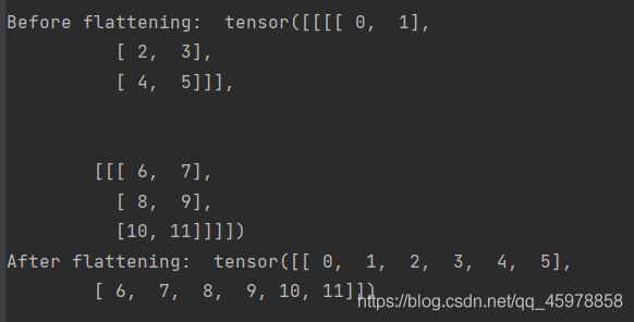
当我们在做2D卷积之类的事情时，这是表示数据的正确方法，这需要空间理解中间特征彼此之间的相对位置。然而，当我们使用完全连接的仿射层来处理图像时，我们希望每个数据点用单个向量表示——分离数据的不同通道、行和列不再有用。因此，我们使用“flatten”操作将每个表示的C x H x W值折叠成一个单独的长向量。下面的flatten函数首先从给定的一批数据中读取N、C、H和W值，然后返回该数据的“视图”。“View”类似于numpy的“重塑”方法)

ln[3]:

def flatten(x):
    N = x.shape[0] # read in N, C, H, W
    return x.view(N, -1)  # "flatten" the C * H * W values into a single vector per image

def test_flatten():
    x = torch.arange(12).view(2, 1, 3, 2)
    print('Before flattening: ', x)
    print('After flattening: ', flatten(x))

test_flatten()

Barebones PyTorch:两层网络
这里我们定义了一个函数two_layer_fc，它执行对一批图像数据的两层全连接ReLU网络的转发。在定义前向传递之后，我们检查它是否会崩溃，并通过网络运行0来生成正确的形状。

您不必在这里编写任何代码，但阅读并理解实现是很重要的
ln[4]:

import torch.nn.functional as F  # useful stateless functions

def two_layer_fc(x, params):
    """
    A fully-connected neural networks; the architecture is:
    NN is fully connected -> ReLU -> fully connected layer.
    Note that this function only defines the forward pass; 
    PyTorch will take care of the backward pass for us.
    
    The input to the network will be a minibatch of data, of shape
    (N, d1, ..., dM) where d1 * ... * dM = D. The hidden layer will have H units,
    and the output layer will produce scores for C classes.
    
    Inputs:
    - x: A PyTorch Tensor of shape (N, d1, ..., dM) giving a minibatch of
      input data.
    - params: A list [w1, w2] of PyTorch Tensors giving weights for the network;
      w1 has shape (D, H) and w2 has shape (H, C).
    
    Returns:
    - scores: A PyTorch Tensor of shape (N, C) giving classification scores for
      the input data x.
    """
    # first we flatten the image
    x = flatten(x)  # shape: [batch_size, C x H x W]
    
    w1, w2 = params
    
    # Forward pass: compute predicted y using operations on Tensors. Since w1 and
    # w2 have requires_grad=True, operations involving these Tensors will cause
    # PyTorch to build a computational graph, allowing automatic computation of
    # gradients. Since we are no longer implementing the backward pass by hand we
    # don't need to keep references to intermediate values.
    # you can also use `.clamp(min=0)`, equivalent to F.relu()
    x = F.relu(x.mm(w1))
    x = x.mm(w2)
    return x
    

def two_layer_fc_test():
    hidden_layer_size = 42
    x = torch.zeros((64, 50), dtype=dtype)  # minibatch size 64, feature dimension 50
    w1 = torch.zeros((50, hidden_layer_size), dtype=dtype)
    w2 = torch.zeros((hidden_layer_size, 10), dtype=dtype)
    scores = two_layer_fc(x, [w1, w2])
    print(scores.size())  # you should see [64, 10]

two_layer_fc_test()

Barebones PyTorch:三层ConvNet

在这里，您将完成函数three_layer_convnet的实现，该函数将执行三层卷积网络的前向传递。像上面一样，我们可以通过在网络中传递0来立即测试我们的实现。网络应具有以下架构:

1.带有channel_1滤波器的卷积层(带偏置)，每个滤波器的形状为KW1 x KH1，零填充为2

2.ReLU

3.带有channel_2滤波器的卷积层(带偏置)，每个滤波器的形状为KW2 x KH2，零填充为1

4.ReLU

5.带有偏差的全连接层，为C类生成分数。

请注意，在我们的全连接层之后，这里没有softmax激活:这是因为PyTorch的交叉熵损失为您执行了softmax激活，通过将该步骤绑定进来，使计算更加高效。
ln[5]:

def three_layer_convnet(x, params):
    """
    Performs the forward pass of a three-layer convolutional network with the
    architecture defined above.

    Inputs:
    - x: A PyTorch Tensor of shape (N, 3, H, W) giving a minibatch of images
    - params: A list of PyTorch Tensors giving the weights and biases for the
      network; should contain the following:
      - conv_w1: PyTorch Tensor of shape (channel_1, 3, KH1, KW1) giving weights
        for the first convolutional layer
      - conv_b1: PyTorch Tensor of shape (channel_1,) giving biases for the first
        convolutional layer
      - conv_w2: PyTorch Tensor of shape (channel_2, channel_1, KH2, KW2) giving
        weights for the second convolutional layer
      - conv_b2: PyTorch Tensor of shape (channel_2,) giving biases for the second
        convolutional layer
      - fc_w: PyTorch Tensor giving weights for the fully-connected layer. Can you
        figure out what the shape should be?
      - fc_b: PyTorch Tensor giving biases for the fully-connected layer. Can you
        figure out what the shape should be?
    
    Returns:
    - scores: PyTorch Tensor of shape (N, C) giving classification scores for x
    """
    conv_w1, conv_b1, conv_w2, conv_b2, fc_w, fc_b = params
    scores = None
    ################################################################################
    # TODO: Implement the forward pass for the three-layer ConvNet.                #
    ################################################################################
    # *****START OF YOUR CODE (DO NOT DELETE/MODIFY THIS LINE)*****
    l1=F.relu_(F.conv2d(x,conv_w1,conv_b1,padding=2))
    l2=F.relu_(F.conv2d(l1,conv_w2,conv_b2,padding=1))
    scores=F.linear(flatten(l2),fc_w.T,fc_b)
    # *****END OF YOUR CODE (DO NOT DELETE/MODIFY THIS LINE)*****
    ################################################################################
    #                                 END OF YOUR CODE                             #
    ################################################################################
    return scores

ln[6]:

def three_layer_convnet_test():
    x = torch.zeros((64, 3, 32, 32), dtype=dtype)  # minibatch size 64, image size [3, 32, 32]

    conv_w1 = torch.zeros((6, 3, 5, 5), dtype=dtype)  # [out_channel, in_channel, kernel_H, kernel_W]
    conv_b1 = torch.zeros((6,))  # out_channel
    conv_w2 = torch.zeros((9, 6, 3, 3), dtype=dtype)  # [out_channel, in_channel, kernel_H, kernel_W]
    conv_b2 = torch.zeros((9,))  # out_channel

    # you must calculate the shape of the tensor after two conv layers, before the fully-connected layer
    fc_w = torch.zeros((9 * 32 * 32, 10))
    fc_b = torch.zeros(10)

    scores = three_layer_convnet(x, [conv_w1, conv_b1, conv_w2, conv_b2, fc_w, fc_b])
    print(scores.size())  # you should see [64, 10]
three_layer_convnet_test()

Barebones PyTorch: 初始化
让我们编写几个实用程序方法来初始化模型的权重矩阵。
random_weight(shape)使用Kaiming normalization方法初始化一个权张量。
Zero_weight (shape)用所有的0初始化一个权张量。用于实例化偏差参数。

random_weight函数使用Kaiming normalization方法，描述如下:
ln[7]:

def random_weight(shape):
    """
    Create random Tensors for weights; setting requires_grad=True means that we
    want to compute gradients for these Tensors during the backward pass.
    We use Kaiming normalization: sqrt(2 / fan_in)
    """
    if len(shape) == 2:  # FC weight
        fan_in = shape[0]
    else:
        fan_in = np.prod(shape[1:]) # conv weight [out_channel, in_channel, kH, kW]
    # randn is standard normal distribution generator. 
    w = torch.randn(shape, device=device, dtype=dtype) * np.sqrt(2. / fan_in)
    w.requires_grad = True
    return w

def zero_weight(shape):
    return torch.zeros(shape, device=device, dtype=dtype, requires_grad=True)

# create a weight of shape [3 x 5]
# you should see the type `torch.cuda.FloatTensor` if you use GPU. 
# Otherwise it should be `torch.FloatTensor`
random_weight((3, 5))

Barebones PyTorch:检查准确性
在训练模型时，我们将使用以下函数来检查模型在训练或验证集上的准确性。
当检查精度时，我们不需要计算任何梯度;因此，当我们计算分数时，不需要PyTorch为我们构建计算图。为了防止图形被构建，我们将计算范围限定在torch.no_grad()上下文管理器
ln[8]:

def check_accuracy_part2(loader, model_fn, params):
    """
    Check the accuracy of a classification model.
    
    Inputs:
    - loader: A DataLoader for the data split we want to check
    - model_fn: A function that performs the forward pass of the model,
      with the signature scores = model_fn(x, params)
    - params: List of PyTorch Tensors giving parameters of the model
    
    Returns: Nothing, but prints the accuracy of the model
    """
    split = 'val' if loader.dataset.train else 'test'
    print('Checking accuracy on the %s set' % split)
    num_correct, num_samples = 0, 0
    with torch.no_grad():
        for x, y in loader:
            x = x.to(device=device, dtype=dtype)  # move to device, e.g. GPU
            y = y.to(device=device, dtype=torch.int64)
            scores = model_fn(x, params)
            _, preds = scores.max(1)
            num_correct += (preds == y).sum()
            num_samples += preds.size(0)
        acc = float(num_correct) / num_samples
        print('Got %d / %d correct (%.2f%%)' % (num_correct, num_samples, 100 * acc))

BareBones PyTorch:训练循环

我们现在可以建立一个基本的训练循环来训练我们的网络。我们将使用无动量的随机梯度下降训练模型。我们用torch.functional.cross_entropy计算损失的交叉熵

训练循环以神经网络函数、初始化参数列表(在本例中为[w1, w2])和学习率作为输入。
ln[9]:

def train_part2(model_fn, params, learning_rate):
    """
    Train a model on CIFAR-10.
    
    Inputs:
    - model_fn: A Python function that performs the forward pass of the model.
      It should have the signature scores = model_fn(x, params) where x is a
      PyTorch Tensor of image data, params is a list of PyTorch Tensors giving
      model weights, and scores is a PyTorch Tensor of shape (N, C) giving
      scores for the elements in x.
    - params: List of PyTorch Tensors giving weights for the model
    - learning_rate: Python scalar giving the learning rate to use for SGD
    
    Returns: Nothing
    """
    for t, (x, y) in enumerate(loader_train):
        # Move the data to the proper device (GPU or CPU)
        x = x.to(device=device, dtype=dtype)
        y = y.to(device=device, dtype=torch.long)

        # Forward pass: compute scores and loss
        scores = model_fn(x, params)
        loss = F.cross_entropy(scores, y)

        # Backward pass: PyTorch figures out which Tensors in the computational
        # graph has requires_grad=True and uses backpropagation to compute the
        # gradient of the loss with respect to these Tensors, and stores the
        # gradients in the .grad attribute of each Tensor.
        loss.backward()

        # Update parameters. We don't want to backpropagate through the
        # parameter updates, so we scope the updates under a torch.no_grad()
        # context manager to prevent a computational graph from being built.
        with torch.no_grad():
            for w in params:
                w -= learning_rate * w.grad

                # Manually zero the gradients after running the backward pass
                w.grad.zero_()

        if t % print_every == 0:
            print('Iteration %d, loss = %.4f' % (t, loss.item()))
            check_accuracy_part2(loader_val, model_fn, params)
            print()

BareBones PyTorch:训练一个双层网络

现在我们可以运行训练循环了。我们需要明确地为完全连通权值w1和w2分配张量。

CIFAR的每个小批有64个例子，所以张量形状为[64,3,32,32]。

压扁后，x形为[64,3 * 32 * 32]。这就是w1的第一个维度的大小。w1的第2维是隐藏层大小，它也将是w2的第1维。

最后，网络的输出是一个10维向量，表示10类以上的概率分布。

您不需要调整任何超参数，但您应该看到，在训练一个时期后，准确率超过40%。
ln[10]:

hidden_layer_size = 4000
learning_rate = 1e-2

w1 = random_weight((3 * 32 * 32, hidden_layer_size))
w2 = random_weight((hidden_layer_size, 10))

train_part2(two_layer_fc, [w1, w2], learning_rate)

Iteration 0, loss = 3.1955
Checking accuracy on the val set
Got 143 / 1000 correct (14.30%)
Iteration 100, loss = 2.1915
Checking accuracy on the val set
Got 336 / 1000 correct (33.60%)
Iteration 200, loss = 2.3473
Checking accuracy on the val set
Got 331 / 1000 correct (33.10%)
Iteration 300, loss = 1.9082
Checking accuracy on the val set
Got 371 / 1000 correct (37.10%)
Iteration 400, loss = 2.0966
Checking accuracy on the val set
Got 406 / 1000 correct (40.60%)
Iteration 500, loss = 1.7127
Checking accuracy on the val set
Got 403 / 1000 correct (40.30%)
Iteration 600, loss = 2.0710
Checking accuracy on the val set
Got 424 / 1000 correct (42.40%)
Iteration 700, loss = 1.6236
Checking accuracy on the val set
Got 433 / 1000 correct (43.30%)

BareBones PyTorch: Training a ConvNet
在下面的代码中，您应该使用上面定义的函数在CIFAR上训练一个三层卷积网络。网络应具有以下架构:

1.带有32个5x5滤波器的卷积层(带偏差)，零填充为2
2.ReLU
3.具有16个3x3滤波器的卷积层(带偏差)，零填充为1
4.ReLU
5.全连接层(带有偏差)计算10个类的分数
你应该使用上面定义的random_weight函数初始化你的权重矩阵，你应该使用上面的zero_weight函数初始化你的偏差向量。
您不需要调优任何超参数，但如果一切正常，您应该在一个epoch之后达到42%以上的精度。
ln[11]:

learning_rate = 3e-3

channel_1 = 32
channel_2 = 16

conv_w1 = None
conv_b1 = None
conv_w2 = None
conv_b2 = None
fc_w = None
fc_b = None

################################################################################
# TODO: Initialize the parameters of a three-layer ConvNet.                    #
################################################################################
# *****START OF YOUR CODE (DO NOT DELETE/MODIFY THIS LINE)*****

conv_w1 = random_weight((channel_1, 3, 5, 5))
conv_b1 = zero_weight((channel_1,))
conv_w2 = random_weight((channel_2, channel_1, 3, 3))
conv_b2 = zero_weight((channel_2,))
fc_w = random_weight((channel_2 * 32 * 32, 10))
fc_b = zero_weight((10,))

# *****END OF YOUR CODE (DO NOT DELETE/MODIFY THIS LINE)*****
################################################################################
#                                 END OF YOUR CODE                             #
################################################################################

params = [conv_w1, conv_b1, conv_w2, conv_b2, fc_w, fc_b]
train_part2(three_layer_convnet, params, learning_rate)

Iteration 0, loss = 3.5806
Checking accuracy on the val set
Got 111 / 1000 correct (11.10%)
Iteration 100, loss = 1.7560
Checking accuracy on the val set
Got 332 / 1000 correct (33.20%)
Iteration 200, loss = 1.7835
Checking accuracy on the val set
Got 372 / 1000 correct (37.20%)
Iteration 300, loss = 1.7980
Checking accuracy on the val set
Got 420 / 1000 correct (42.00%)
Iteration 400, loss = 1.7919
Checking accuracy on the val set
Got 423 / 1000 correct (42.30%)
Iteration 500, loss = 1.5235
Checking accuracy on the val set
Got 452 / 1000 correct (45.20%)
Iteration 600, loss = 1.4753
Checking accuracy on the val set
Got 436 / 1000 correct (43.60%)
Iteration 700, loss = 1.6224
Checking accuracy on the val set
Got 455 / 1000 correct (45.50%)

第三部分,PyTorch Module API

Barebone PyTorch要求我们手工跟踪所有参数张量。这对于具有少量张量的小型网络来说是很好的，但是在较大的网络中跟踪数十或数百张量会非常不方便而且容易出错。

PyTorch提供nn.Module为您定义任意的网络架构，同时跟踪每个可学习的参数。在第二部分中，我们自己实现了SGD。PyTorch还提供了torch.optim，它实现了所有常见的优化器，如RMSProp、Adagrad和Adam。它甚至支持近似的二阶方法，如L-BFGS!。

要使用Module API，请遵循以下步骤:

1.子类nn.Module。给网络类起一个直观的名字，比如TwoLayerFC。

2.在构造函数__init__()中，将需要的所有层定义为类属性。层对象如nn.Linear，nn.Conv2d模块的子类和包含可学习的参数，这样你就不必自己实例化原始张量。神经网络。模块将为您跟踪这些内部参数。请参考文档了解关于几十个内置层的更多信息。警告:不要忘记首先调用super().init() !

3.在forward()方法中，定义网络的连通性。你应该使用__init__中定义的属性作为函数调用，以张量作为输入，并输出“转换”的张量。不要在forward()中创建任何带有可学习参数的新层!所有这些都必须在__init__中提前声明。

在你定义了你的Module子类之后，你可以实例化它作为一个对象，并调用它，就像第二部分的NN forward函数一样。

Module API:两层网络
下面是一个2层全连接网络的具体例子:
ln[12]:

class TwoLayerFC(nn.Module):
    def __init__(self, input_size, hidden_size, num_classes):
        super().__init__()
        # assign layer objects to class attributes
        self.fc1 = nn.Linear(input_size, hidden_size)
        # nn.init package contains convenient initialization methods
        # http://pytorch.org/docs/master/nn.html#torch-nn-init 
        nn.init.kaiming_normal_(self.fc1.weight)
        self.fc2 = nn.Linear(hidden_size, num_classes)
        nn.init.kaiming_normal_(self.fc2.weight)
    
    def forward(self, x):
        # forward always defines connectivity
        x = flatten(x)
        scores = self.fc2(F.relu(self.fc1(x)))
        return scores

def test_TwoLayerFC():
    input_size = 50
    x = torch.zeros((64, input_size), dtype=dtype)  # minibatch size 64, feature dimension 50
    model = TwoLayerFC(input_size, 42, 10)
    scores = model(x)
    print(scores.size())  # you should see [64, 10]
test_TwoLayerFC()

Module API:Three-Layer ConvNet

ln[13]:

class ThreeLayerConvNet(nn.Module):
    def __init__(self, in_channel, channel_1, channel_2, num_classes):
        super().__init__()
        ########################################################################
        # TODO: Set up the layers you need for a three-layer ConvNet with the  #
        # architecture defined above.                                          #
        ########################################################################
        # *****START OF YOUR CODE (DO NOT DELETE/MODIFY THIS LINE)*****

        self.conv1 = nn.Conv2d(in_channel, channel_1, 5, padding=2)
        nn.init.kaiming_normal_(self.conv1.weight)
        self.conv2 = nn.Conv2d(channel_1, channel_2, 3, padding=1)
        nn.init.kaiming_normal_(self.conv2.weight)
        self.fc = nn.Linear(channel_2*32*32, num_classes)
        nn.init.kaiming_normal_(self.fc.weight)

        # *****END OF YOUR CODE (DO NOT DELETE/MODIFY THIS LINE)*****
        ########################################################################
        #                          END OF YOUR CODE                            #       
        ########################################################################

    def forward(self, x):
        scores = None
        ########################################################################
        # TODO: Implement the forward function for a 3-layer ConvNet. you      #
        # should use the layers you defined in __init__ and specify the        #
        # connectivity of those layers in forward()                            #
        ########################################################################
        # *****START OF YOUR CODE (DO NOT DELETE/MODIFY THIS LINE)*****
        c1 = F.relu(self.conv1(x))
        c2 = F.relu(self.conv2(c1))
        scores = self.fc(flatten(c2))

        # *****END OF YOUR CODE (DO NOT DELETE/MODIFY THIS LINE)*****
        ########################################################################
        #                             END OF YOUR CODE                         #
        ########################################################################
        return scores


def test_ThreeLayerConvNet():
    x = torch.zeros((64, 3, 32, 32), dtype=dtype)  # minibatch size 64, image size [3, 32, 32]
    model = ThreeLayerConvNet(in_channel=3, channel_1=12, channel_2=8, num_classes=10)
    scores = model(x)
    print(scores.size())  # you should see [64, 10]
test_ThreeLayerConvNet()

Module API:Check Accuracy

ln[14]:

def check_accuracy_part34(loader, model):
    if loader.dataset.train:
        print('Checking accuracy on validation set')
    else:
        print('Checking accuracy on test set')   
    num_correct = 0
    num_samples = 0
    model.eval()  # set model to evaluation mode
    with torch.no_grad():
        for x, y in loader:
            x = x.to(device=device, dtype=dtype)  # move to device, e.g. GPU
            y = y.to(device=device, dtype=torch.long)
            scores = model(x)
            _, preds = scores.max(1)
            num_correct += (preds == y).sum()
            num_samples += preds.size(0)
        acc = float(num_correct) / num_samples
        print('Got %d / %d correct (%.2f)' % (num_correct, num_samples, 100 * acc))

Module API:Training Loop

ln[15]:

def train_part34(model, optimizer, epochs=1):
    """
    Train a model on CIFAR-10 using the PyTorch Module API.
    
    Inputs:
    - model: A PyTorch Module giving the model to train.
    - optimizer: An Optimizer object we will use to train the model
    - epochs: (Optional) A Python integer giving the number of epochs to train for
    
    Returns: Nothing, but prints model accuracies during training.
    """
    model = model.to(device=device)  # move the model parameters to CPU/GPU
    for e in range(epochs):
        for t, (x, y) in enumerate(loader_train):
            model.train()  # put model to training mode
            x = x.to(device=device, dtype=dtype)  # move to device, e.g. GPU
            y = y.to(device=device, dtype=torch.long)

            scores = model(x)
            loss = F.cross_entropy(scores, y)

            # Zero out all of the gradients for the variables which the optimizer
            # will update.
            optimizer.zero_grad()

            # This is the backwards pass: compute the gradient of the loss with
            # respect to each  parameter of the model.
            loss.backward()

            # Actually update the parameters of the model using the gradients
            # computed by the backwards pass.
            optimizer.step()

            if t % print_every == 0:
                print('Iteration %d, loss = %.4f' % (t, loss.item()))
                check_accuracy_part34(loader_val, model)
                print()

Module API:Train a Two-Layer Network

ln[16]:

hidden_layer_size = 4000
learning_rate = 1e-2
model = TwoLayerFC(3 * 32 * 32, hidden_layer_size, 10)
optimizer = optim.SGD(model.parameters(), lr=learning_rate)

train_part34(model, optimizer)

Iteration 0, loss = 3.4061
Checking accuracy on validation set
Got 157 / 1000 correct (15.70)
Iteration 100, loss = 2.3327
Checking accuracy on validation set
Got 334 / 1000 correct (33.40)
Iteration 200, loss = 1.6200
Checking accuracy on validation set
Got 379 / 1000 correct (37.90)
Iteration 300, loss = 1.9143
Checking accuracy on validation set
Got 367 / 1000 correct (36.70)
Iteration 400, loss = 1.5516
Checking accuracy on validation set
Got 395 / 1000 correct (39.50)
Iteration 500, loss = 1.3761
Checking accuracy on validation set
Got 440 / 1000 correct (44.00)
Iteration 600, loss = 1.7966
Checking accuracy on validation set
Got 420 / 1000 correct (42.00)
Iteration 700, loss = 2.0415
Checking accuracy on validation set
Got 451 / 1000 correct (45.10)

模块API:Train a Three-Layer ConvNet
ln[17]:

learning_rate = 3e-3
channel_1 = 32
channel_2 = 16

model = None
optimizer = None
################################################################################
# TODO: Instantiate your ThreeLayerConvNet model and a corresponding optimizer #
################################################################################
# *****START OF YOUR CODE (DO NOT DELETE/MODIFY THIS LINE)*****

model = ThreeLayerConvNet(in_channel=3, channel_1=channel_1, channel_2=channel_2, num_classes=10)
optimizer = optim.SGD(model.parameters(), lr=learning_rate)

# *****END OF YOUR CODE (DO NOT DELETE/MODIFY THIS LINE)*****
################################################################################
#                                 END OF YOUR CODE                             
################################################################################

train_part34(model, optimizer)

Iteration 0, loss = 3.8634
Checking accuracy on validation set
Got 128 / 1000 correct (12.80)
Iteration 100, loss = 1.7045
Checking accuracy on validation set
Got 349 / 1000 correct (34.90)
Iteration 200, loss = 1.6994
Checking accuracy on validation set
Got 365 / 1000 correct (36.50)
Iteration 300, loss = 1.3177
Checking accuracy on validation set
Got 404 / 1000 correct (40.40)
Iteration 400, loss = 1.5059
Checking accuracy on validation set
Got 451 / 1000 correct (45.10)
Iteration 500, loss = 1.4896
Checking accuracy on validation set
Got 443 / 1000 correct (44.30)
Iteration 600, loss = 1.2600
Checking accuracy on validation set
Got 460 / 1000 correct (46.00)
Iteration 700, loss = 1.5156
Checking accuracy on validation set
Got 482 / 1000 correct (48.20)

第四部分。PyTorch Sequential API

第三部分介绍了PyTorch模块API，它允许您定义任意可学习的层及其连接性。

对于像前馈层堆栈这样的简单模型，你仍然需要通过3个步骤:子类nn.Module，在__init__中为层分配类属性，并在forward()中逐个调用每一层。有没有更方便的方法?

幸运的是，PyTorch提供了一个名为nn.Sequential的容器模块，它将上述步骤合并为一个步骤。它不像nn.Module那么灵活，因为不能指定比前馈堆栈更复杂的拓扑，但它对于许多用例来说已经足够了。

Sequential API:两层网络

让我们看看如何用nn.Sequential来重写我们的两层全连接网络的例子，并使用上面定义的训练循环对其进行训练。

同样，你不需要在这里调整任何超参数，但你应该在一个时期的训练后达到40%以上的准确率。
ln[18]:

# We need to wrap `flatten` function in a module in order to stack it
# in nn.Sequential
class Flatten(nn.Module):
    def forward(self, x):
        return flatten(x)

hidden_layer_size = 4000
learning_rate = 1e-2

model = nn.Sequential(
    Flatten(),
    nn.Linear(3 * 32 * 32, hidden_layer_size),
    nn.ReLU(),
    nn.Linear(hidden_layer_size, 10),
)

# you can use Nesterov momentum in optim.SGD
optimizer = optim.SGD(model.parameters(), lr=learning_rate,
                     momentum=0.9, nesterov=True)

train_part34(model, optimizer)

Iteration 0, loss = 2.4063
Checking accuracy on validation set
Got 163 / 1000 correct (16.30)
Iteration 100, loss = 1.7647
Checking accuracy on validation set
Got 368 / 1000 correct (36.80)
Iteration 200, loss = 1.7949
Checking accuracy on validation set
Got 383 / 1000 correct (38.30)
Iteration 300, loss = 1.5341
Checking accuracy on validation set
Got 430 / 1000 correct (43.00)
Iteration 400, loss = 1.9970
Checking accuracy on validation set
Got 407 / 1000 correct (40.70)
Iteration 500, loss = 1.7346
Checking accuracy on validation set
Got 445 / 1000 correct (44.50)
Iteration 600, loss = 1.8268
Checking accuracy on validation set
Got 420 / 1000 correct (42.00)
Iteration 700, loss = 1.6695
Checking accuracy on validation set
Got 471 / 1000 correct (47.10)

Sequential API:三层卷积网络
ln[19]:

channel_1 = 32
channel_2 = 16
learning_rate = 1e-2

model = None
optimizer = None

################################################################################
# TODO: Rewrite the 2-layer ConvNet with bias from Part III with the           #
# Sequential API.                                                              #
################################################################################
# *****START OF YOUR CODE (DO NOT DELETE/MODIFY THIS LINE)*****

in_channel = 3
num_classes = 10

model = nn.Sequential(
    nn.Conv2d(in_channel, channel_1, 5, padding=2),
    nn.ReLU(),
    nn.Conv2d(channel_1, channel_2, 3, padding=1),
    nn.ReLU(),
    Flatten(),
    nn.Linear(channel_2*32*32, num_classes)
)

# you can use Nesterov momentum in optim.SGD
optimizer = optim.SGD(model.parameters(), lr=learning_rate,
                     momentum=0.9, nesterov=True)

# *****END OF YOUR CODE (DO NOT DELETE/MODIFY THIS LINE)*****
################################################################################
#                                 END OF YOUR CODE                             
################################################################################

train_part34(model, optimizer)

Iteration 0, loss = 2.2869
Checking accuracy on validation set
Got 118 / 1000 correct (11.80)
Iteration 100, loss = 1.6109
Checking accuracy on validation set
Got 447 / 1000 correct (44.70)
Iteration 200, loss = 1.4254
Checking accuracy on validation set
Got 466 / 1000 correct (46.60)
Iteration 300, loss = 1.2840
Checking accuracy on validation set
Got 533 / 1000 correct (53.30)
Iteration 400, loss = 1.3280
Checking accuracy on validation set
Got 537 / 1000 correct (53.70)
Iteration 500, loss = 1.1625
Checking accuracy on validation set
Got 558 / 1000 correct (55.80)
Iteration 600, loss = 1.2066
Checking accuracy on validation set
Got 548 / 1000 correct (54.80)
Iteration 700, loss = 1.1647
Checking accuracy on validation set
Got 574 / 1000 correct (57.40)

第五部分CIFAR-10开放式挑战

在本节中，您可以在CIFAR-10上试验您喜欢的任何ConvNet架构。

现在，您的工作是用架构、超参数、损失函数和优化器进行实验，以训练一个模型，在10个Iteration内在CIFAR-10验证集上达到至少70%的精度。您可以使用上面提到的check_accuracy和train函数。你可以使用任何一个nn,Module或nn.Sequential API。

在笔记本的最后描述一下你做了什么。

下面是每个组件的官方API文档。注意:我们在类中称为“空间批处理标准化”的在PyTorch中称为“BatchNorm2D”。
Layers in torch.nn package: http://pytorch.org/docs/stable/nn.html
Activations: http://pytorch.org/docs/stable/nn.html#non-linear-activations
Loss functions: http://pytorch.org/docs/stable/nn.html#loss-functions
Optimizers: http://pytorch.org/docs/stable/optim.html

祝你训练愉快!
ln[20]:

################################################################################
# TODO:                                                                        #         
# Experiment with any architectures, optimizers, and hyperparameters.          #
# Achieve AT LEAST 70% accuracy on the *validation set* within 10 epochs.      #
#                                                                              #
# Note that you can use the check_accuracy function to evaluate on either      #
# the test set or the validation set, by passing either loader_test or         #
# loader_val as the second argument to check_accuracy. You should not touch    #
# the test set until you have finished your architecture and  hyperparameter   #
# tuning, and only run the test set once at the end to report a final value.   #
################################################################################
model = None
optimizer = None

# *****START OF YOUR CODE (DO NOT DELETE/MODIFY THIS LINE)*****

channel_1 = 32
channel_2 = 128
channel_3 = 256
channel_4 = 256
channel_5 = 128

hidden_1 = 64
hidden_2 = 64
num_classes = 10

learning_rate = 1e-2

in_channel = 3
pool_kernel = 2
pool_stride = 2

dropout = 0.2

model = nn.Sequential(
    # Simplified AlexNet
    nn.Conv2d(in_channel, channel_1, 5, padding=0), # H*W = 28*28
    # Here 28 = (32-5+0)//1 +1 
    nn.ReLU(inplace=True),
    nn.Dropout2d(p=dropout),
    nn.MaxPool2d(kernel_size=2),# H*W = 14*14
    
    nn.BatchNorm2d(channel_1),
    nn.Conv2d(channel_1, channel_2, 3, padding=1), # H*W = 14*14
    nn.ReLU(inplace=True),
    nn.Dropout2d(p=dropout),
    nn.MaxPool2d(kernel_size=2), # H*W = 7*7
    
    nn.BatchNorm2d(channel_2),
    nn.Conv2d(channel_2, channel_3, 3, padding=1), # H*W = 7*7
    nn.ReLU(inplace=True),
    nn.Dropout2d(p=dropout),
    nn.Conv2d(channel_3, channel_4, 3, padding=1), # H*W = 7*7
    nn.ReLU(inplace=True),
    nn.Dropout2d(p=dropout),
    nn.Conv2d(channel_4, channel_5, 3, padding=1), # H*W = 7*7
    nn.ReLU(inplace=True),
    
    Flatten(),
    nn.Linear(channel_5*7*7, hidden_1),
    nn.ReLU(inplace=True),
#     nn.Dropout2d(p=dropout),
    nn.Linear(hidden_1, hidden_2),
    nn.ReLU(inplace=True),
#     nn.Dropout2d(p=dropout),
    nn.Linear(hidden_2, num_classes),
)

optimizer = optim.Adam(model.parameters())

# *****END OF YOUR CODE (DO NOT DELETE/MODIFY THIS LINE)*****
################################################################################
#                                 END OF YOUR CODE                             
################################################################################

# You should get at least 70% accuracy
train_part34(model, optimizer, epochs=10)

最后的实践：
ln[21]:

best_model = model
check_accuracy_part34(loader_test, best_model)

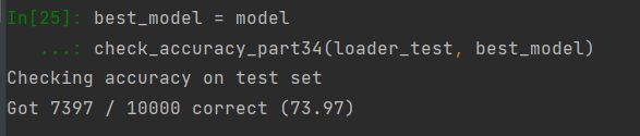
勉强过关吧家人们