【Python机器学习项目】项目一:心脏病二分类问题
使用机器学习预测心脏病
根据一些病理学属性预测心脏病
特别说明:
-
开新坑啦!本系列共2个项目,难度不大,特别适合新手入坑
-
由于本项目只是系列课程的第一个项目,所以很多细节不深挖,仅做示范,在第二个项目中再完善。
以下为整体思路概述
1. 问题定义
给定一个病人的临床诊断,能否预测他们是否患有心脏病?
2. 数据来源
https://archive.ics.uci.edu/ml/datasets/Heart+Disease
3. 评估
期望准确率达到95%
4. 特征和标签
数据字典
- age: age in years
- sex: sex (1 = male; 0 = female)
- cp: chest pain type
- – Value 0: typical angina
- – Value 1: atypical angina
- – Value 2: non-anginal pain
- – Value 3: asymptomatic
- trestbps: resting blood pressure (in mm Hg on admission to the hospital)
- chol: serum cholestoral in mg/dl
- fbs: (fasting blood sugar > 120 mg/dl) (1 = true; 0 = false)
- restecg: resting electrocardiographic results
- – Value 0: normal
- – Value 1: having ST-T wave abnormality (T wave inversions and/or ST elevation or depression of > 0.05 mV)
- – Value 2: showing probable or definite left ventricular hypertrophy by Estes’ criteria
- thalach: maximum heart rate achieved
- exang: exercise induced angina (1 = yes; 0 = no)
- oldpeak = ST depression induced by exercise relative to rest
- slope: the slope of the peak exercise ST segment
- – Value 0: upsloping
- – Value 1: flat
- – Value 2: downsloping
- ca: number of major vessels (0-3) colored by flourosopy
- thal: 0 = normal; 1 = fixed defect; 2 = reversable defect
- target: 0 = no disease, 1 = disease
0. 导包
# EDA
import numpy as np
import pandas as pd
import matplotlib.pyplot as plt
import seaborn as sns
from scipy import stats
sns.set()
plt.rcParams['font.sans-serif'] = ['SimHei']
plt.rcParams['axes.unicode_minus'] = False
%config InlineBackend.figure_config = 'svg'

# sklearn模型
from sklearn.neighbors import KNeighborsClassifier
from sklearn.linear_model import LogisticRegression
from sklearn.ensemble import RandomForestClassifier

# 模型评估
from sklearn.model_selection import train_test_split, cross_val_score
from sklearn.model_selection import RandomizedSearchCV, GridSearchCV
from sklearn.metrics import confusion_matrix, classification_report
from sklearn.metrics import precision_score, recall_score, f1_score
from sklearn.metrics import plot_roc_curve
载入数据
hd_df = pd.read_csv('heart-disease.csv')
hd_df.shape
(303, 14)
1. EDA
了解更多有关这个数据集的信息,成为该数据集的懂王
- 要解决什么问题?
- 都有些什么数据,要怎么处理?
- 有无缺失值,如何处理?
- 有无异常值,如何处理?
- 如何通过创建衍生特征、处理和筛选现有特征得到更多信息?
hd_df.head()
| age | sex | cp | trestbps | chol | fbs | restecg | thalach | exang | oldpeak | slope | ca | thal | target | |
|---|---|---|---|---|---|---|---|---|---|---|---|---|---|---|
| 0 | 63 | 1 | 3 | 145 | 233 | 1 | 0 | 150 | 0 | 2.3 | 0 | 0 | 1 | 1 |
| 1 | 37 | 1 | 2 | 130 | 250 | 0 | 1 | 187 | 0 | 3.5 | 0 | 0 | 2 | 1 |
| 2 | 41 | 0 | 1 | 130 | 204 | 0 | 0 | 172 | 0 | 1.4 | 2 | 0 | 2 | 1 |
| 3 | 56 | 1 | 1 | 120 | 236 | 0 | 1 | 178 | 0 | 0.8 | 2 | 0 | 2 | 1 |
| 4 | 57 | 0 | 0 | 120 | 354 | 0 | 1 | 163 | 1 | 0.6 | 2 | 0 | 2 | 1 |
hd_df.tail()
| age | sex | cp | trestbps | chol | fbs | restecg | thalach | exang | oldpeak | slope | ca | thal | target | |
|---|---|---|---|---|---|---|---|---|---|---|---|---|---|---|
| 298 | 57 | 0 | 0 | 140 | 241 | 0 | 1 | 123 | 1 | 0.2 | 1 | 0 | 3 | 0 |
| 299 | 45 | 1 | 3 | 110 | 264 | 0 | 1 | 132 | 0 | 1.2 | 1 | 0 | 3 | 0 |
| 300 | 68 | 1 | 0 | 144 | 193 | 1 | 1 | 141 | 0 | 3.4 | 1 | 2 | 3 | 0 |
| 301 | 57 | 1 | 0 | 130 | 131 | 0 | 1 | 115 | 1 | 1.2 | 1 | 1 | 3 | 0 |
| 302 | 57 | 0 | 1 | 130 | 236 | 0 | 0 | 174 | 0 | 0.0 | 1 | 1 | 2 | 0 |
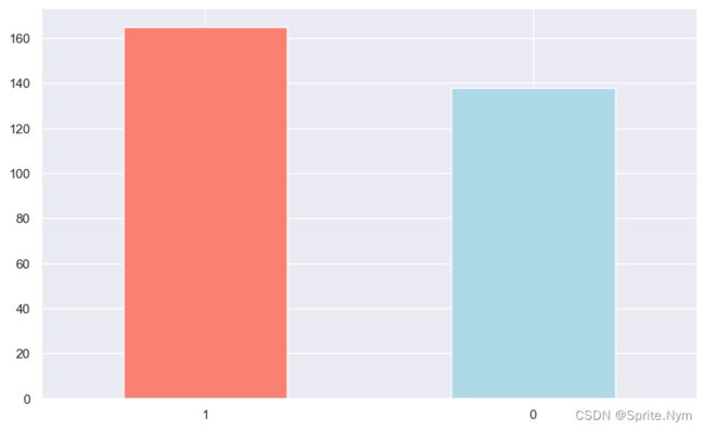
# 查看样本分布
targets = hd_df['target'].value_counts()
targets
1    165
0    138
Name: target, dtype: int64
targets.plot(
    kind='bar',
    color=['salmon', 'lightblue'],
    figsize=(10,6)
)
plt.xticks(rotation=0)
plt.show()
hd_df.info()
RangeIndex: 303 entries, 0 to 302
Data columns (total 14 columns):
 #   Column    Non-Null Count  Dtype
---  ------    --------------  -----
 0   age       303 non-null    int64
 1   sex       303 non-null    int64
 2   cp        303 non-null    int64
 3   trestbps  303 non-null    int64
 4   chol      303 non-null    int64
 5   fbs       303 non-null    int64
 6   restecg   303 non-null    int64
 7   thalach   303 non-null    int64
 8   exang     303 non-null    int64
 9   oldpeak   303 non-null    float64
 10  slope     303 non-null    int64
 11  ca        303 non-null    int64
 12  thal      303 non-null    int64
 13  target    303 non-null    int64
dtypes: float64(1), int64(13)
memory usage: 33.3 KB
# 查看缺失值
hd_df.isna().sum()
age         0
sex         0
cp          0
trestbps    0
chol        0
fbs         0
restecg     0
thalach     0
exang       0
oldpeak     0
slope       0
ca          0
thal        0
target      0
dtype: int64
# 查看描述性统计信息
hd_df.describe([0.01, 0.25, 0.5, 0.75, 0.99]).T
| count | mean | std | min | 1% | 25% | 50% | 75% | 99% | max | |
|---|---|---|---|---|---|---|---|---|---|---|
| age | 303.0 | 54.366337 | 9.082101 | 29.0 | 35.00 | 47.5 | 55.0 | 61.0 | 71.00 | 77.0 |
| sex | 303.0 | 0.683168 | 0.466011 | 0.0 | 0.00 | 0.0 | 1.0 | 1.0 | 1.00 | 1.0 |
| cp | 303.0 | 0.966997 | 1.032052 | 0.0 | 0.00 | 0.0 | 1.0 | 2.0 | 3.00 | 3.0 |
| trestbps | 303.0 | 131.623762 | 17.538143 | 94.0 | 100.00 | 120.0 | 130.0 | 140.0 | 180.00 | 200.0 |
| chol | 303.0 | 246.264026 | 51.830751 | 126.0 | 149.00 | 211.0 | 240.0 | 274.5 | 406.74 | 564.0 |
| fbs | 303.0 | 0.148515 | 0.356198 | 0.0 | 0.00 | 0.0 | 0.0 | 0.0 | 1.00 | 1.0 |
| restecg | 303.0 | 0.528053 | 0.525860 | 0.0 | 0.00 | 0.0 | 1.0 | 1.0 | 1.98 | 2.0 |
| thalach | 303.0 | 149.646865 | 22.905161 | 71.0 | 95.02 | 133.5 | 153.0 | 166.0 | 191.96 | 202.0 |
| exang | 303.0 | 0.326733 | 0.469794 | 0.0 | 0.00 | 0.0 | 0.0 | 1.0 | 1.00 | 1.0 |
| oldpeak | 303.0 | 1.039604 | 1.161075 | 0.0 | 0.00 | 0.0 | 0.8 | 1.6 | 4.20 | 6.2 |
| slope | 303.0 | 1.399340 | 0.616226 | 0.0 | 0.00 | 1.0 | 1.0 | 2.0 | 2.00 | 2.0 |
| ca | 303.0 | 0.729373 | 1.022606 | 0.0 | 0.00 | 0.0 | 0.0 | 1.0 | 4.00 | 4.0 |
| thal | 303.0 | 2.313531 | 0.612277 | 0.0 | 1.00 | 2.0 | 2.0 | 3.0 | 3.00 | 3.0 |
| target | 303.0 | 0.544554 | 0.498835 | 0.0 | 0.00 | 0.0 | 1.0 | 1.0 | 1.00 | 1.0 |
查看性别和标签之间的关系
hd_df['sex'].value_counts()
1    207
0     96
Name: sex, dtype: int64
# cross_tab改进版函数
def to_cross_tab(origin_df, index_name, col_name):
    df = pd.crosstab(origin_df[index_name], origin_df[col_name])
    df['rate'] = df.iloc[:,1] / (df.iloc[:,0] + df.iloc[:,1])
    return df
sex_target_df = to_cross_tab(hd_df, 'target', 'sex')
sex_target_df
| sex | 0 | 1 | rate |
|---|---|---|---|
| target | |||
| 0 | 24 | 114 | 0.750000 |
| 1 | 72 | 93 | 0.449275 |
# 方便绘图的函数
def to_plot(df, title, xlabel, ylabel, legend):
    df.plot(
    kind='bar',
    color=['lightblue', 'salmon'],
    figsize=(10,6)
)
    plt.title(title)
    plt.xlabel(xlabel)
    plt.ylabel(ylabel)
    plt.xticks(rotation=0)
    plt.legend(legend)
    plt.show()
to_plot(sex_target_df[[0,1]], '按性别统计的心脏病概率', '0 = 女生, 1 = 男生', '总人数', ['未得病', '得病'])
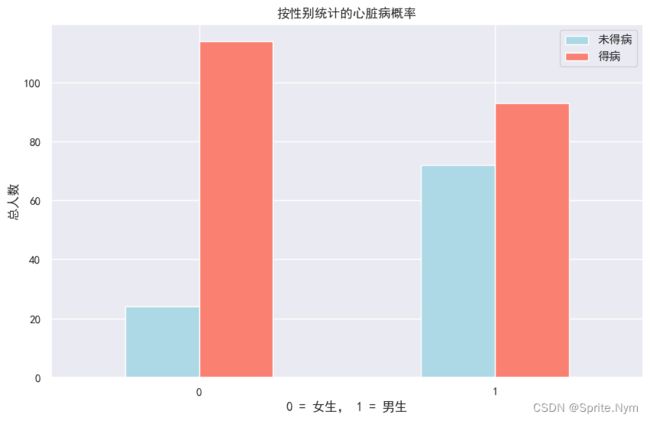
明显女性发病率高得多
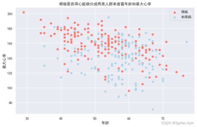
查看得病/未得病两类人中年龄和最大心率的关系
plt.figure(figsize=(10,6))

# 查看得病人群
plt.scatter(hd_df['age'][hd_df['target']==1],
            hd_df['thalach'][hd_df['target']==1],
            c='salmon'
)

# 查看未得病人群
plt.scatter(hd_df['age'][hd_df['target']==0],
            hd_df['thalach'][hd_df['target']==0],
            c='lightblue'
)

# 说明
plt.title('根据是否得心脏病分成两类人群来查看年龄和最大心率')
plt.xlabel('年龄')
plt.ylabel('最大心率')
plt.legend(['得病', '未得病'])

plt.show()
# 查看年龄分布
hd_df['age'].hist()
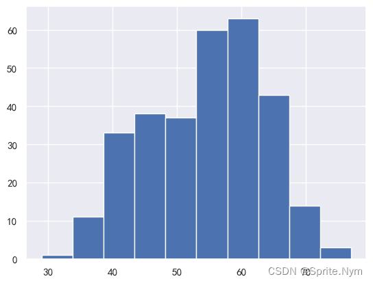
# 做正态性检验
stats.normaltest(hd_df['age'])
NormaltestResult(statistic=8.74798581312778, pvalue=0.012600826063683705)
年龄符合正态分布
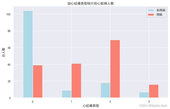
查看心绞痛类型和标签之间的关系
- cp: chest pain type
- – Value 0: typical angina
- – Value 1: atypical angina
- – Value 2: non-anginal pain
- – Value 3: asymptomatic
cp_target_df = to_cross_tab(hd_df, 'cp', 'target')
cp_target_df
| target | 0 | 1 | rate |
|---|---|---|---|
| cp | |||
| 0 | 104 | 39 | 0.272727 |
| 1 | 9 | 41 | 0.820000 |
| 2 | 18 | 69 | 0.793103 |
| 3 | 7 | 16 | 0.695652 |
to_plot(cp_target_df[[0,1]], '按心绞痛类型统计的心脏病人数', '心绞痛类型', '总人数', ['未得病', '得病'])
# 相关系数矩阵
corr_matrix = hd_df.corr()
corr_matrix
| age | sex | cp | trestbps | chol | fbs | restecg | thalach | exang | oldpeak | slope | ca | thal | target | |
|---|---|---|---|---|---|---|---|---|---|---|---|---|---|---|
| age | 1.000000 | -0.098447 | -0.068653 | 0.279351 | 0.213678 | 0.121308 | -0.116211 | -0.398522 | 0.096801 | 0.210013 | -0.168814 | 0.276326 | 0.068001 | -0.225439 |
| sex | -0.098447 | 1.000000 | -0.049353 | -0.056769 | -0.197912 | 0.045032 | -0.058196 | -0.044020 | 0.141664 | 0.096093 | -0.030711 | 0.118261 | 0.210041 | -0.280937 |
| cp | -0.068653 | -0.049353 | 1.000000 | 0.047608 | -0.076904 | 0.094444 | 0.044421 | 0.295762 | -0.394280 | -0.149230 | 0.119717 | -0.181053 | -0.161736 | 0.433798 |
| trestbps | 0.279351 | -0.056769 | 0.047608 | 1.000000 | 0.123174 | 0.177531 | -0.114103 | -0.046698 | 0.067616 | 0.193216 | -0.121475 | 0.101389 | 0.062210 | -0.144931 |
| chol | 0.213678 | -0.197912 | -0.076904 | 0.123174 | 1.000000 | 0.013294 | -0.151040 | -0.009940 | 0.067023 | 0.053952 | -0.004038 | 0.070511 | 0.098803 | -0.085239 |
| fbs | 0.121308 | 0.045032 | 0.094444 | 0.177531 | 0.013294 | 1.000000 | -0.084189 | -0.008567 | 0.025665 | 0.005747 | -0.059894 | 0.137979 | -0.032019 | -0.028046 |
| restecg | -0.116211 | -0.058196 | 0.044421 | -0.114103 | -0.151040 | -0.084189 | 1.000000 | 0.044123 | -0.070733 | -0.058770 | 0.093045 | -0.072042 | -0.011981 | 0.137230 |
| thalach | -0.398522 | -0.044020 | 0.295762 | -0.046698 | -0.009940 | -0.008567 | 0.044123 | 1.000000 | -0.378812 | -0.344187 | 0.386784 | -0.213177 | -0.096439 | 0.421741 |
| exang | 0.096801 | 0.141664 | -0.394280 | 0.067616 | 0.067023 | 0.025665 | -0.070733 | -0.378812 | 1.000000 | 0.288223 | -0.257748 | 0.115739 | 0.206754 | -0.436757 |
| oldpeak | 0.210013 | 0.096093 | -0.149230 | 0.193216 | 0.053952 | 0.005747 | -0.058770 | -0.344187 | 0.288223 | 1.000000 | -0.577537 | 0.222682 | 0.210244 | -0.430696 |
| slope | -0.168814 | -0.030711 | 0.119717 | -0.121475 | -0.004038 | -0.059894 | 0.093045 | 0.386784 | -0.257748 | -0.577537 | 1.000000 | -0.080155 | -0.104764 | 0.345877 |
| ca | 0.276326 | 0.118261 | -0.181053 | 0.101389 | 0.070511 | 0.137979 | -0.072042 | -0.213177 | 0.115739 | 0.222682 | -0.080155 | 1.000000 | 0.151832 | -0.391724 |
| thal | 0.068001 | 0.210041 | -0.161736 | 0.062210 | 0.098803 | -0.032019 | -0.011981 | -0.096439 | 0.206754 | 0.210244 | -0.104764 | 0.151832 | 1.000000 | -0.344029 |
| target | -0.225439 | -0.280937 | 0.433798 | -0.144931 | -0.085239 | -0.028046 | 0.137230 | 0.421741 | -0.436757 | -0.430696 | 0.345877 | -0.391724 | -0.344029 | 1.000000 |
plt.figure(figsize=(14, 10))
sns.heatmap(
    corr_matrix,
    vmin=-1,
    annot=True,
    linewidth=5,
    fmt='.2f',
    cmap='YlGnBu'
)
plt.show()
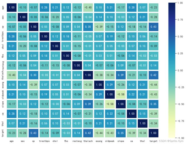
这个相关性看起来还是比较好的,大部分特征和标签之间都有一定的相关性,且特征之间也没有相关性>0.8的需要排除。当然,真的想看相关性还得分类别变量和连续值变量,连续值变量又得做正态检验。
3. 建模
hd_df.head()
| age | sex | cp | trestbps | chol | fbs | restecg | thalach | exang | oldpeak | slope | ca | thal | target | |
|---|---|---|---|---|---|---|---|---|---|---|---|---|---|---|
| 0 | 63 | 1 | 3 | 145 | 233 | 1 | 0 | 150 | 0 | 2.3 | 0 | 0 | 1 | 1 |
| 1 | 37 | 1 | 2 | 130 | 250 | 0 | 1 | 187 | 0 | 3.5 | 0 | 0 | 2 | 1 |
| 2 | 41 | 0 | 1 | 130 | 204 | 0 | 0 | 172 | 0 | 1.4 | 2 | 0 | 2 | 1 |
| 3 | 56 | 1 | 1 | 120 | 236 | 0 | 1 | 178 | 0 | 0.8 | 2 | 0 | 2 | 1 |
| 4 | 57 | 0 | 0 | 120 | 354 | 0 | 1 | 163 | 1 | 0.6 | 2 | 0 | 2 | 1 |
X = hd_df.drop(columns=['target'])
y = hd_df['target']
# 设置随机种子,便于其他人重复实验
np.random.seed(13)

# 划分训练集和测试集
X_train, X_test, y_train, y_test = train_test_split(X, y, test_size=0.2)
依次使用逻辑斯蒂回归、KNN、随机森林
# 创建字典
models = {
    'lr': LogisticRegression(),
    'knn': KNeighborsClassifier(),
    'rf': RandomForestClassifier()
}

# 一个简单的试探性fit和score的函数
def fit_and_score(models, X_train, X_test, y_train, y_test):
    np.random.seed(13)
    model_score = {}
    for name, model in models.items():
        model.fit(X_train, y_train)
        model_score[name] = model.score(X_test, y_test)
    return model_score
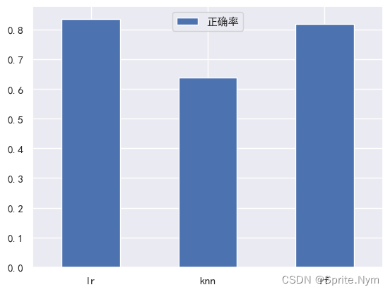
model_scores = fit_and_score(models, X_train, X_test, y_train, y_test)
model_scores
{'lr': 0.8360655737704918, 'knn': 0.639344262295082, 'rf': 0.819672131147541}
模型比较
model_compare = pd.DataFrame(model_scores, index=['正确率'])
model_compare.T.plot(kind='bar')
plt.xticks(rotation=0)
plt.show()
接下来做什么?
- 超参数优化
- 特征重要性
- 混淆矩阵
- 交叉验证
- 精确率
- 召回率
- F1 score
- 分类报告
- ROC
- AUC
# knn调参(假装不会GSCV和RSCV)
train_scores = []
test_scores = []

neighbors = range(1, 21)

knn = KNeighborsClassifier()
for i in n_neighbors:
    knn.set_params(n_neighbors=i)
    knn.fit(X_train, y_train)
    train_scores.append(knn.score(X_train, y_train))
    test_scores.append(knn.score(X_test, y_test))
train_scores
[1.0,
 0.8016528925619835,
 0.8057851239669421,
 0.7603305785123967,
 0.768595041322314,
 0.7355371900826446,
 0.7396694214876033,
 0.71900826446281,
 0.7024793388429752,
 0.6900826446280992,
 0.7107438016528925,
 0.6859504132231405,
 0.7024793388429752,
 0.6776859504132231,
 0.6942148760330579,
 0.6859504132231405,
 0.6694214876033058,
 0.6859504132231405,
 0.7024793388429752,
 0.7066115702479339]
test_scores
[0.6065573770491803,
 0.4426229508196721,
 0.5737704918032787,
 0.5409836065573771,
 0.639344262295082,
 0.6557377049180327,
 0.6065573770491803,
 0.6721311475409836,
 0.6557377049180327,
 0.6557377049180327,
 0.6885245901639344,
 0.6885245901639344,
 0.6885245901639344,
 0.7377049180327869,
 0.7213114754098361,
 0.7213114754098361,
 0.7213114754098361,
 0.7049180327868853,
 0.7377049180327869,
 0.7377049180327869]
plt.plot(neighbors, train_scores, label='Train score')
plt.plot(neighbors, test_scores, label='Test score')
plt.xticks(range(1,21,1))
plt.xlabel('n_neighbors参数值')
plt.ylabel('正确率')
plt.legend()
plt.show()
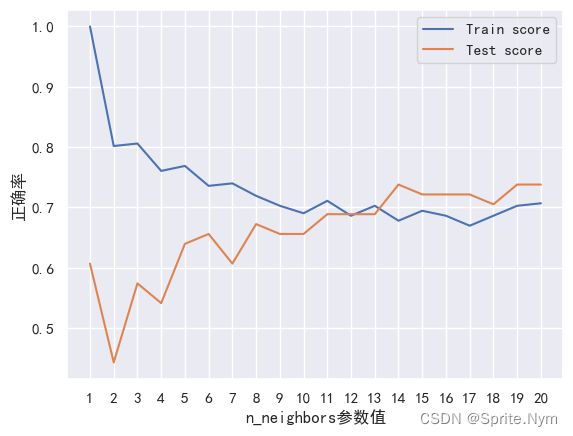
knn最高分也没达到80%正确率,放弃
使用RandomizedSearchCV调参
# 逻辑斯蒂回归
# 由于主要是想找最优C值,其他参数就不设置了,并且这里使用np.logspace故意把C值分布得开一些,因为完全不知道在哪里取得最优值
log_reg_grid = {
    'C':np.logspace(-4, 4, 20),
    'solver': ['liblinear']
}

# 随机森林
rf_grid = {
    'n_estimators': np.arange(10, 1000, 50),
    'max_depth': [None, 3, 5, 10],
    'min_samples_split': np.arange(2, 20, 2),
    'min_samples_leaf': np.arange(1, 20, 2)
}
np.random.seed(13)

# 实例化RSCV对象
rs_log_reg = RandomizedSearchCV(
    LogisticRegression(),
    param_distributions=log_reg_grid,
    cv=5,
    n_iter=20,
    verbose=True
)
# fit
rs_log_reg.fit(X_train, y_train)
Fitting 5 folds for each of 20 candidates, totalling 100 fits
RandomizedSearchCV(cv=5, estimator=LogisticRegression(), n_iter=20,In a Jupyter environment, please rerun this cell to show the HTML representation or trust the notebook.param_distributions={'C': array([1.00000000e-04, 2.63665090e-04, 6.95192796e-04, 1.83298071e-03, 4.83293024e-03, 1.27427499e-02, 3.35981829e-02, 8.85866790e-02, 2.33572147e-01, 6.15848211e-01, 1.62377674e+00, 4.28133240e+00, 1.12883789e+01, 2.97635144e+01, 7.84759970e+01, 2.06913808e+02, 5.45559478e+02, 1.43844989e+03, 3.79269019e+03, 1.00000000e+04]), 'solver': ['liblinear']}, verbose=True)
On GitHub, the HTML representation is unable to render, please try loading this page with nbviewer.org.
RandomizedSearchCV(cv=5, estimator=LogisticRegression(), n_iter=20,
               param_distributions={'C': array([1.00000000e-04, 2.63665090e-04, 6.95192796e-04, 1.83298071e-03,
   4.83293024e-03, 1.27427499e-02, 3.35981829e-02, 8.85866790e-02,
   2.33572147e-01, 6.15848211e-01, 1.62377674e+00, 4.28133240e+00,
   1.12883789e+01, 2.97635144e+01, 7.84759970e+01, 2.06913808e+02,
   5.45559478e+02, 1.43844989e+03, 3.79269019e+03, 1.00000000e+04]),
                                    'solver': ['liblinear']},
verbose=True)LogisticRegression()
LogisticRegression()
rs_log_reg.best_params_
{'solver': 'liblinear', 'C': 1.623776739188721}
rs_log_reg.score(X_test, y_test)
0.819672131147541
负提升,难绷,由于只是第一个项目,对调参仅做展示,就不管了
np.random.seed(13)

# 实例化RSCV对象
rs_rf = RandomizedSearchCV(
    RandomForestClassifier(),
    param_distributions=rf_grid,
    cv=5,
    n_iter=20,
    verbose=True
)
# fit
rs_rf.fit(X_train, y_train)
Fitting 5 folds for each of 20 candidates, totalling 100 fits
RandomizedSearchCV(cv=5, estimator=RandomForestClassifier(), n_iter=20,In a Jupyter environment, please rerun this cell to show the HTML representation or trust the notebook.param_distributions={'max_depth': [None, 3, 5, 10], 'min_samples_leaf': array([ 1, 3, 5, 7, 9, 11, 13, 15, 17, 19]), 'min_samples_split': array([ 2, 4, 6, 8, 10, 12, 14, 16, 18]), 'n_estimators': array([ 10, 60, 110, 160, 210, 260, 310, 360, 410, 460, 510, 560, 610, 660, 710, 760, 810, 860, 910, 960])}, verbose=True)
On GitHub, the HTML representation is unable to render, please try loading this page with nbviewer.org.
RandomizedSearchCV(cv=5, estimator=RandomForestClassifier(), n_iter=20,
               param_distributions={'max_depth': [None, 3, 5, 10],
                                    'min_samples_leaf': array([ 1,  3,  5,  7,  9, 11, 13, 15, 17, 19]),
                                    'min_samples_split': array([ 2,  4,  6,  8, 10, 12, 14, 16, 18]),
                                    'n_estimators': array([ 10,  60, 110, 160, 210, 260, 310, 360, 410, 460, 510, 560, 610,
   660, 710, 760, 810, 860, 910, 960])},
verbose=True)RandomForestClassifier()
RandomForestClassifier()
rs_rf.best_params_
{'n_estimators': 310,
 'min_samples_split': 16,
 'min_samples_leaf': 9,
 'max_depth': None}
rs_rf.score(X_test, y_test)
0.8360655737704918
有轻微提升
使用GSCV调参
这次稍微多用点参数
log_reg_grid = {
    'C':np.logspace(-4, 4, 30),
    'solver': ['liblinear', 'sag', 'saga', 'newton-cg', 'lbfgs'],
    'penalty': ['l1', 'l2']
}

# 实例化RSCV对象
gs_log_reg = GridSearchCV(
    LogisticRegression(),
    param_grid=log_reg_grid,
    cv=5,
    verbose=True
)
# fit
gs_log_reg.fit(X_train, y_train)
GridSearchCV(cv=5, estimator=LogisticRegression(),In a Jupyter environment, please rerun this cell to show the HTML representation or trust the notebook.param_grid={'C': array([1.00000000e-04, 1.88739182e-04, 3.56224789e-04, 6.72335754e-04, 1.26896100e-03, 2.39502662e-03, 4.52035366e-03, 8.53167852e-03, 1.61026203e-02, 3.03919538e-02, 5.73615251e-02, 1.08263673e-01, 2.04335972e-01, 3.85662042e-01, 7.27895384e-01, 1.37382380e+00, 2.59294380e+00, 4.89390092e+00, 9.23670857e+00, 1.74332882e+01, 3.29034456e+01, 6.21016942e+01, 1.17210230e+02, 2.21221629e+02, 4.17531894e+02, 7.88046282e+02, 1.48735211e+03, 2.80721620e+03, 5.29831691e+03, 1.00000000e+04]), 'penalty': ['l1', 'l2'], 'solver': ['liblinear', 'sag', 'saga', 'newton-cg', 'lbfgs']}, verbose=True)
On GitHub, the HTML representation is unable to render, please try loading this page with nbviewer.org.
GridSearchCV(cv=5, estimator=LogisticRegression(),
         param_grid={'C': array([1.00000000e-04, 1.88739182e-04, 3.56224789e-04, 6.72335754e-04,
   1.26896100e-03, 2.39502662e-03, 4.52035366e-03, 8.53167852e-03,
   1.61026203e-02, 3.03919538e-02, 5.73615251e-02, 1.08263673e-01,
   2.04335972e-01, 3.85662042e-01, 7.27895384e-01, 1.37382380e+00,
   2.59294380e+00, 4.89390092e+00, 9.23670857e+00, 1.74332882e+01,
   3.29034456e+01, 6.21016942e+01, 1.17210230e+02, 2.21221629e+02,
   4.17531894e+02, 7.88046282e+02, 1.48735211e+03, 2.80721620e+03,
   5.29831691e+03, 1.00000000e+04]),
                     'penalty': ['l1', 'l2'],
                     'solver': ['liblinear', 'sag', 'saga', 'newton-cg',
                                'lbfgs']},
verbose=True)LogisticRegression()
LogisticRegression()
gs_log_reg.best_params_
{'C': 221.22162910704503, 'penalty': 'l2', 'solver': 'lbfgs'}
和之前的分数一样…
gs_log_reg.score(X_test, y_test)
0.819672131147541
4. 评估
y_pred = gs_log_reg.predict(X_test)
y_pred
array([0, 1, 1, 1, 1, 0, 0, 0, 1, 0, 1, 1, 0, 0, 1, 1, 1, 0, 0, 0, 0, 0,
       1, 0, 1, 1, 1, 1, 0, 0, 1, 0, 0, 1, 0, 0, 1, 0, 1, 1, 1, 0, 0, 1,
       0, 1, 1, 0, 1, 1, 1, 0, 1, 1, 1, 0, 0, 1, 1, 1, 1], dtype=int64)
y_test
203    0
30     1
58     1
90     1
119    1
      ..
249    0
135    1
41     1
67     1
148    1
Name: target, Length: 61, dtype: int64
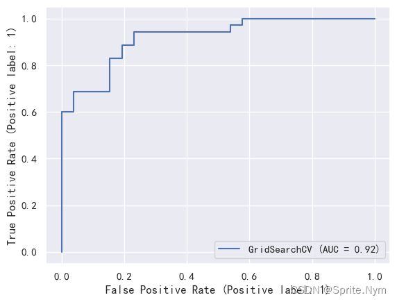
plot_roc_curve(gs_log_reg, X_test, y_test)
y_pred==1
array([False,  True,  True,  True,  True, False, False, False,  True,
       False,  True,  True, False, False,  True,  True,  True, False,
       False, False, False, False,  True, False,  True,  True,  True,
        True, False, False,  True, False, False,  True, False, False,
        True, False,  True,  True,  True, False, False,  True, False,
        True,  True, False,  True,  True,  True, False,  True,  True,
        True, False, False,  True,  True,  True,  True])
# 混淆矩阵
def to_confusion_matrix(y_test, y_pred):
    return pd.DataFrame(
        data=confusion_matrix(y_test, y_pred),
        index=pd.MultiIndex.from_product([['y_test'], [0, 1]]),
        columns=pd.MultiIndex.from_product([['y_pred'], [0, 1]])
    )
cf_matrix = to_confusion_matrix(y_test, y_pred)
cf_matrix
| y_pred | |||
|---|---|---|---|
| 0 | 1 | ||
| y_test | 0 | 21 | 5 |
| 1 | 6 | 29 | |
# 分类报告
print(classification_report(y_test, y_pred))
              precision    recall  f1-score   support

           0       0.78      0.81      0.79        26
           1       0.85      0.83      0.84        35

    accuracy                           0.82        61
   macro avg       0.82      0.82      0.82        61
weighted avg       0.82      0.82      0.82        61
利用交叉验证评估模型
利用交叉验证计算精确率、召回率、F1值
gs_log_reg.best_params_
{'C': 221.22162910704503, 'penalty': 'l2', 'solver': 'lbfgs'}
# 重新实例化逻辑斯蒂回归模型
clf = LogisticRegression(
    C=221.22162910704503,
    penalty='l2',
    solver='lbfgs'
)
# 交叉验证正确率
cv_acc = cross_val_score(
    clf,
    X,
    y,
    cv=5,
    scoring='accuracy'
)
cv_acc
array([0.81967213, 0.83606557, 0.85245902, 0.83333333, 0.75 ])
cv_acc = np.mean(cv_acc)
cv_acc
0.8183060109289617
# 交叉验证精确率
cv_precision = cross_val_score(
    clf,
    X,
    y,
    cv=5,
    scoring='precision'
)
cv_precision = np.mean(cv_precision)
cv_precision
0.8088942275474784
# 交叉验证召回率
cv_recall = cross_val_score(
    clf,
    X,
    y,
    cv=5,
    scoring='recall'
)
cv_recall = np.mean(cv_recall)
cv_recall
0.8787878787878787
# 交叉验证F1值
cv_f1 = cross_val_score(
    clf,
    X,
    y,
    cv=5,
    scoring='f1'
)
cv_f1 = np.mean(cv_f1)
cv_f1
0.8413377274453797
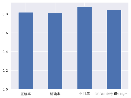
# 可视化
cv_metrics = pd.DataFrame(
    {'正确率': cv_acc,
     '精确率': cv_precision,
     '召回率': cv_recall,
     'f1值': cv_f1
    },
    index=[0]
)
cv_metrics.T.plot(
    kind='bar',
    legend=False
)
plt.xticks(rotation=0)
plt.show()
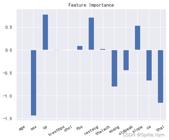
5. 评估特征重要性
clf.fit(X_train, y_train)
LogisticRegression(C=221.22162910704503)
clf.coef_
array([[ 0.00513208, -1.43253864,  0.78004753, -0.01083726, -0.0019836 ,
         0.0976912 ,  0.71562367,  0.03049414, -0.80027663, -0.44530236,
         0.53599288, -0.66841624, -1.15804589]])
feature_dict = dict(zip(hd_df.columns, clf.coef_[0]))
feature_dict
{'age': 0.005132076982516595,
 'sex': -1.4325386407347098,
 'cp': 0.7800475335340353,
 'trestbps': -0.010837256399792251,
 'chol': -0.001983600334944071,
 'fbs': 0.09769119644464817,
 'restecg': 0.7156236671955836,
 'thalach': 0.030494138473504826,
 'exang': -0.8002766264626233,
 'oldpeak': -0.44530236148020047,
 'slope': 0.5359928831085665,
 'ca': -0.6684162375711792,
 'thal': -1.158045891987526}
feature_df = pd.DataFrame(feature_dict, index=['feature_importance'])
feature_df.T.plot(
    kind='bar',
    title='Feature Importance',
    legend=False,
)
plt.xticks(rotation=30)
plt.show()
6. 继续实验
如果没有达到预期目标(比如这次定的95%正确率),则继续研究:
- 还能收集更多数据吗?因为机器学习需要数据
- 能不能换一个更好的模型?比如XGB、CatBoost
- 可以继续调参优化吗?
如果已经达到了预期目标,想想:
怎么给其他人汇报工作结果?