FigDraw 21. SCI文章中绘图之三维散点图 (plot3D)

点击关注，桓峰基因

---

桓峰基因公众号推出基于R语言绘图教程并配有视频在线教程，目前整理出来的教程目录如下：

FigDraw 1. SCI 文章的灵魂 之 简约优雅的图表配色

FigDraw 2. SCI 文章绘图必备 R 语言基础

FigDraw 3. SCI 文章绘图必备 R 数据转换

FigDraw 4. SCI 文章绘图之散点图 (Scatter)

FigDraw 5. SCI 文章绘图之柱状图 (Barplot)

FigDraw 6. SCI 文章绘图之箱线图 (Boxplot)

FigDraw 7. SCI 文章绘图之折线图 (Lineplot)

FigDraw 8. SCI 文章绘图之饼图 (Pieplot)

FigDraw 9. SCI 文章绘图之韦恩图 (Vennplot)

FigDraw 10. SCI 文章绘图之直方图 (HistogramPlot)

FigDraw 11. SCI 文章绘图之小提琴图 (ViolinPlot)

FigDraw 12. SCI 文章绘图之相关性矩阵图(Correlation Matrix)

FigDraw 13. SCI 文章绘图之桑葚图及文章复现(Sankey)

FigDraw 14. SCI 文章绘图之和弦图及文章复现（Chord Diagram)

FigDraw 15. SCI 文章绘图之多组学圈图(OmicCircos)

FigDraw 16. SCI 文章绘图之树形图(Dendrogram)

FigDraw 17. SCI 文章绘图之主成分绘图(pca3d)

FigDraw 18. SCI 文章绘图之矩形树状图 (treemap)

FigDraw 19. SCI 文章中绘图之坡度图(Slope Chart)

FigDraw 20. SCI文章中绘图之马赛克图 (mosaic)

三维散点图就是在由3个变量确定的三维空间中研究变量之间的关系，由于同时考虑了3个变量，常常可以发现在两维图形中发现不了的信息。

前 言

三维数据绘制到三维坐标系中，通常称其为三维散点图，即用在三维X-Y-Z图上针对一个或多个数据序列绘出三个度量的一种图表。

软件包安装

R 中scatterplot3d包的scatterplot3d()函数、rgl包的plot3d()函数、plot3D包的scatter3D()函数等都可以绘制三维散点图。

下面将从 plot3D 包的函数scatter3D()入手，一步步带你完成三维散点图的绘制。本文内容丰富，希望大家都能学到自己想要的内容。

if(!require(plot3D))
  install.packages("plot3D")

实例操作

1. 三维球体

library(plot3D)
library(scales)
library(RColorBrewer)
library(fields)
# save plotting parameters
pm <- par("mfrow")

## ======================================================================= A
## sphere
## =======================================================================

par(mfrow = c(1, 1))
M <- mesh(seq(0, 2 * pi, length.out = 100), seq(0, pi, length.out = 100))
u <- M$x
v <- M$y

x <- cos(u) * sin(v)
y <- sin(u) * sin(v)
z <- cos(v)

# full panels of box are drawn (bty = 'f')
scatter3D(x, y, z, pch = ".", col = "red", bty = "f", cex = 2, colkey = FALSE)

2. 不同类型

par(mfrow = c(2, 2))
z <- seq(0, 10, 0.2)
x <- cos(z)
y <- sin(z) * z

# greyish background for the boxtype (bty = 'g')
scatter3D(x, y, z, phi = 0, bty = "g", pch = 20, cex = 2, ticktype = "detailed")
# add another point
scatter3D(x = 0, y = 0, z = 0, add = TRUE, colkey = FALSE, pch = 18, cex = 3, col = "black")

# add text
text3D(x = cos(1:10), y = (sin(1:10) * (1:10) - 1), z = 1:10, colkey = FALSE, add = TRUE,
    labels = LETTERS[1:10], col = c("black", "red"))

# line plot
scatter3D(x, y, z, phi = 0, bty = "g", type = "l", ticktype = "detailed", lwd = 4)

# points and lines
scatter3D(x, y, z, phi = 0, bty = "g", type = "b", ticktype = "detailed", pch = 20,
    cex = c(0.5, 1, 1.5))

# vertical lines
scatter3D(x, y, z, phi = 0, bty = "g", type = "h", ticktype = "detailed")

3. 带有自信区间

x <- runif(20)
y <- runif(20)
z <- runif(20)

par(mfrow = c(1, 1))
CI <- list(z = matrix(nrow = length(x), ncol = 2, data = rep(0.05, times = 2 * length(x))))

# greyish background for the boxtype (bty = 'g')
scatter3D(x, y, z, phi = 0, bty = "g", CI = CI, col = gg.col(100), pch = 18, cex = 2,
    ticktype = "detailed", xlim = c(0, 1), ylim = c(0, 1), zlim = c(0, 1))

# add new set of points
x <- runif(20)
y <- runif(20)
z <- runif(20)

CI2 <- list(x = matrix(nrow = length(x), ncol = 2, data = rep(0.05, 2 * length(x))),
    z = matrix(nrow = length(x), ncol = 2, data = rep(0.05, 2 * length(x))))

scatter3D(x, y, z, CI = CI2, add = TRUE, col = "red", pch = 16)

4. 带有表面和CI

par(mfrow = c(1, 1))

# surface = volcano
M <- mesh(1:nrow(volcano), 1:ncol(volcano))

# 100 points above volcano
N <- 100
xs <- runif(N) * 87
ys <- runif(N) * 61
zs <- runif(N) * 50 + 154

# scatter + surface
scatter3D(xs, ys, zs, ticktype = "detailed", pch = 16, bty = "f", xlim = c(1, 87),
    ylim = c(1, 61), zlim = c(94, 215), surf = list(x = M$x, y = M$y, z = volcano,
        NAcol = "grey", shade = 0.1))

## ======================================================================= A
## surface and CI
## =======================================================================

par(mfrow = c(1, 1))
M <- mesh(seq(0, 2 * pi, length = 30), (1:30)/100)
z <- with(M, sin(x) + y)

# points 'sampled'
N <- 30
xs <- runif(N) * 2 * pi
ys <- runif(N) * 0.3

zs <- sin(xs) + ys + rnorm(N) * 0.3

CI <- list(z = matrix(nrow = length(xs), data = rep(0.3, 2 * length(xs))), lwd = 3)

# facets = NA makes a transparent surface; borders are black
scatter3D(xs, ys, zs, ticktype = "detailed", pch = 16, xlim = c(0, 2 * pi), ylim = c(0,
    0.3), zlim = c(-1.5, 1.5), CI = CI, theta = 20, phi = 30, cex = 2, surf = list(x = M$x,
    y = M$y, z = z, border = "black", facets = NA))

5. 滴漏至贴合表面

with(mtcars, {

    # linear regression
    fit <- lm(mpg ~ wt + disp)

    # predict values on regular xy grid
    wt.pred <- seq(1.5, 5.5, length.out = 30)
    disp.pred <- seq(71, 472, length.out = 30)
    xy <- expand.grid(wt = wt.pred, disp = disp.pred)

    mpg.pred <- matrix(nrow = 30, ncol = 30, data = predict(fit, newdata = data.frame(xy),
        interval = "prediction")[, 1])

    # fitted points for droplines to surface
    fitpoints <- predict(fit)

    scatter3D(z = mpg, x = wt, y = disp, pch = 18, cex = 2, theta = 20, phi = 20,
        ticktype = "detailed", xlab = "wt", ylab = "disp", zlab = "mpg", surf = list(x = wt.pred,
            y = disp.pred, z = mpg.pred, facets = NA, fit = fitpoints), main = "mtcars")

})

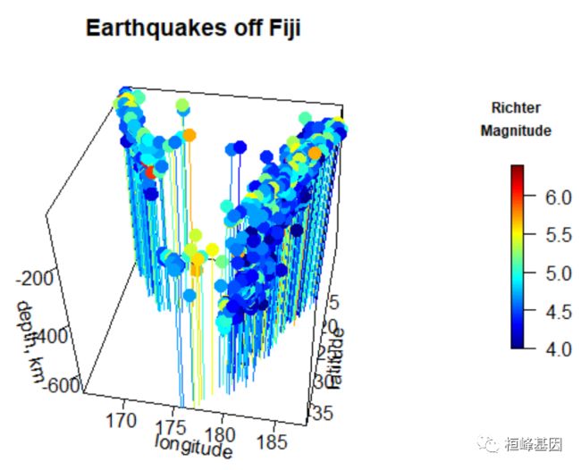
6. 两种方法来制作地震数据集的散点3D

par(mfrow = c(1, 1))
# first way, use vertical spikes (type = 'h')
with(quakes, scatter3D(x = long, y = lat, z = -depth, colvar = mag, pch = 16, cex = 1.5,
    xlab = "longitude", ylab = "latitude", zlab = "depth, km", clab = c("Richter",
        "Magnitude"), main = "Earthquakes off Fiji", ticktype = "detailed", type = "h",
    theta = 10, d = 2, colkey = list(length = 0.5, width = 0.5, cex.clab = 0.75)))

# second way: add dots on bottom and left panel before the scatters are drawn,
# add small dots on basal plane and on the depth plane
panelfirst <- function(pmat) {
    zmin <- min(-quakes$depth)
    XY <- trans3D(quakes$long, quakes$lat, z = rep(zmin, nrow(quakes)), pmat = pmat)
    scatter2D(XY$x, XY$y, colvar = quakes$mag, pch = ".", cex = 2, add = TRUE, colkey = FALSE)

    xmin <- min(quakes$long)
    XY <- trans3D(x = rep(xmin, nrow(quakes)), y = quakes$lat, z = -quakes$depth,
        pmat = pmat)
    scatter2D(XY$x, XY$y, colvar = quakes$mag, pch = ".", cex = 2, add = TRUE, colkey = FALSE)
}

with(quakes, scatter3D(x = long, y = lat, z = -depth, colvar = mag, pch = 16, cex = 1.5,
    xlab = "longitude", ylab = "latitude", zlab = "depth, km", clab = c("Richter",
        "Magnitude"), main = "Earthquakes off Fiji", ticktype = "detailed", panel.first = panelfirst,
    theta = 10, d = 2, colkey = list(length = 0.5, width = 0.5, cex.clab = 0.75)))

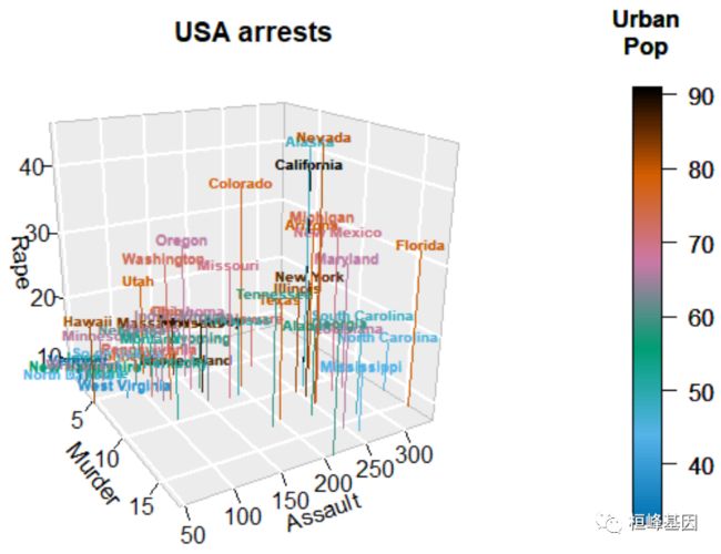
7. text3D and scatter3D

text3D

with(USArrests, text3D(Murder, Assault, Rape, colvar = UrbanPop, col = gg.col(100),
    theta = 60, phi = 20, xlab = "Murder", ylab = "Assault", zlab = "Rape", main = "USA arrests",
    labels = rownames(USArrests), cex = 0.6, bty = "g", ticktype = "detailed", d = 2,
    clab = c("Urban", "Pop"), adj = 0.5, font = 2))
with(USArrests, scatter3D(Murder, Assault, Rape - 1, colvar = UrbanPop, col = gg.col(100),
    type = "h", pch = ".", add = TRUE))

8. 原点缩放

# display axis ranges
getplist()[c("xlim", "ylim", "zlim")]
## $xlim
## [1]  0.8 17.4
## 
## $ylim
## [1]  45 337
## 
## $zlim
## [1]  7.3 46.0

# choose suitable ranges
plotdev(xlim = c(0, 10), ylim = c(40, 150), zlim = c(7, 25))

9. text3D to label x- and y axis

par(mfrow = c(1, 1))
hist3D(x = 1:5, y = 1:4, z = VADeaths, bty = "g", phi = 20, theta = -60, xlab = "",
    ylab = "", zlab = "", main = "VADeaths", col = "#0072B2", border = "black", shade = 0.8,
    ticktype = "detailed", space = 0.15, d = 2, cex.axis = 1e-09)

text3D(x = 1:5, y = rep(0.5, 5), z = rep(3, 5), labels = rownames(VADeaths), add = TRUE,
    adj = 0)
text3D(x = rep(1, 4), y = 1:4, z = rep(0, 4), labels = colnames(VADeaths), add = TRUE,
    adj = 1)

其他的例子

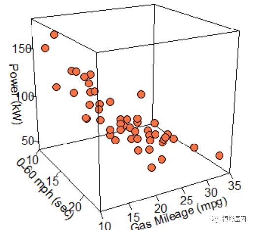
例子 1

df<-read.csv("ThreeD_Scatter_Data.csv",header=T)
head(df)
##   mph Gas_Mileage Power Weight Engine_Displacement
## 1  23          19    69    821              3687.7
## 2  13          17    80   1287              4261.4
## 3  13          22    55   1535              1983.2
## 4  22          34    55   1037              1770.1
## 5  14          29    55   1082              1589.8
## 6  19          26    49   1285              1294.8
pmar <- par(mar = c(5.1, 4.1, 4.1, 6.1))
with(df, scatter3D(x = mph, y = Gas_Mileage, z = Power, #bgvar = mag,
                   pch = 21, cex = 1.5,col="black",bg="#F57446",
                   xlab = "0-60 mph (sec)",
                   ylab = "Gas Mileage (mpg)",
                   zlab = "Power (kW)", 
                   zlim=c(40,180),
                   ticktype = "detailed",bty = "f",box = TRUE,
                   #panel.first = panelfirst,
                   theta = 60, phi = 20, d=3,
                   colkey = FALSE)#list(length = 0.5, width = 0.5, cex.clab = 0.75))
)

例子 2

colormap <- colorRampPalette(rev(brewer.pal(11,'RdYlGn')))(100)#

index <- ceiling(((prc <- 0.7 * df$Power/ diff(range(df$Power))) - min(prc) + 0.3)*100)
for (i in seq(1,length(index)) ){
  prc[i]=colormap[index[i]]
}
pmar <- par(mar = c(5.1, 4.1, 4.1, 6.1))
with(df, scatter3D(x = mph, y = Gas_Mileage, z = Power, #bgvar = mag,
                   pch = 21, cex = 1.5,col="black",bg=prc,
                   xlab = "0-60 mph (sec)",
                   ylab = "Gas Mileage (mpg)",
                   zlab = "Power (kW)", 
                   zlim=c(40,180),
                   ticktype = "detailed",bty = "f",box = TRUE,
                   #panel.first = panelfirst,
                   theta = 60, phi = 20, d=3,
                   colkey = FALSE)#list(length = 0.5, width = 0.5, cex.clab = 0.75))
)
colkey (col=colormap,clim=range(df$Power),clab = "Power", add=TRUE, length=0.5,side = 4)

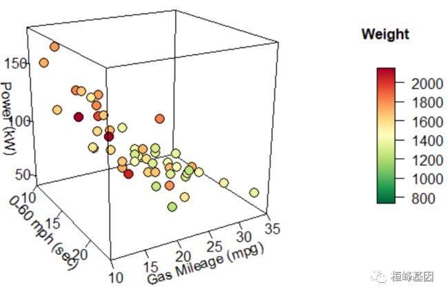
例子 3

index <- ceiling(((prc <- 0.7 * df$Weight/ diff(range(df$Weight))) - min(prc) + 0.3)*100)
for (i in seq(1,length(index)) ){
  prc[i]=colormap[index[i]]
}
pmar <- par(mar = c(5.1, 4.1, 4.1, 6.1))
with(df, scatter3D(x = mph, y = Gas_Mileage, z = Power, #bgvar = mag,
                   pch = 21, cex = 1.5,col="black",bg=prc,
                   xlab = "0-60 mph (sec)",
                   ylab = "Gas Mileage (mpg)",
                   zlab = "Power (kW)", 
                   zlim=c(40,180),
                   ticktype = "detailed",bty = "f",box = TRUE,
                   #panel.first = panelfirst,
                   theta = 60, phi = 20, d=3,
                   colkey = FALSE)#list(length = 0.5, width = 0.5, cex.clab = 0.75))
)
colkey (col=colormap,clim=range(df$Weight),clab = "Weight", add=TRUE, length=0.5,side = 4)

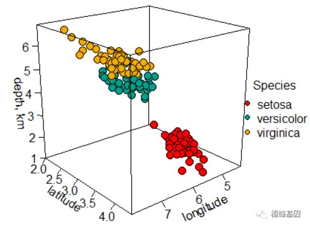
例子 4

library(wesanderson)
pmar <- par(mar = c(5.1, 4.1, 4.1, 7.1))
colors0 <-  wes_palette(n=3, name="Darjeeling1")
colors <- colors0[as.numeric(iris$Species)]
with(iris, scatter3D(x = Sepal.Length, y = Sepal.Width, z = Petal.Length, #bgvar = mag,
                     pch = 21, cex = 1.5,col="black",bg=colors,
                     xlab = "longitude", ylab = "latitude",
                     zlab = "depth, km", 
                     ticktype = "detailed",bty = "f",box = TRUE,
                     #panel.first = panelfirst,
                     theta = 140, phi = 20, d=3,
                     colkey = FALSE)#list(length = 0.5, width = 0.5, cex.clab = 0.75))
)

legend("right",title =  "Species",legend=c("setosa", "versicolor", "virginica"),pch=21,
       cex=1,y.intersp=1,pt.bg = colors0,bg="white",bty="n")

软件包里面自带的例子，我这里都展示了一遍为了方便大家选择适合自己的图形，另外需要代码的将这期教程转发朋友圈，并配文“学生信，找桓峰基因，铸造成功的你！”即可获得！

桓峰基因，铸造成功的您！

有想进生信交流群的老师可以扫最后一个二维码加微信，备注“单位+姓名+目的”，有些想发广告的就免打扰吧，还得费力气把你踢出去！

References:

1. 张杰. R 语言数据可视化之美 专业图表绘制指南

2. plot3d(): http://www.rforscience.com/rpackages