Python3《机器学习实战》学习笔记(六):Logistic回归实战篇之预测病马死亡率
一、随机梯度上升算法
原来:
我们使用的数据集一共有100个样本。那么,dataMatrix就是一个1003的矩阵。每次计算h的时候,都要计算dataMatrixweights这个矩阵乘法运算,要进行1003次乘法运算和1002次加法运算。同理,更新回归系数(最优参数)weights时,也需要用到整个数据集,要进行矩阵乘法运算。总而言之,该方法处理100个左右的数据集时尚可,但如果有数十亿样本和成千上万的特征,那么该方法的计算复杂度就太高了。
改进:
改进之处在于,alpha在每次迭代的时候都会调整,并且,虽然alpha会随着迭代次数不断减小,但永远不会减小到0,因为这里还存在一个常数项。必须这样做的原因是为了保证在多次迭代之后新数据仍然具有一定的影响。如果需要处理的问题是动态变化的,那么可以适当加大上述常数项,来确保新的值获得更大的回归系数。另一点值得注意的是,在降低alpha的函数中,alpha每次减少1/(j+i),其中j是迭代次数,i是样本点的下标。第二个改进的地方在于跟新回归系数(最优参数)时,只使用一个样本点,并且选择的样本点是随机的,每次迭代不使用已经用过的样本点。这样的方法,就有效地减少了计算量,并保证了回归效果。
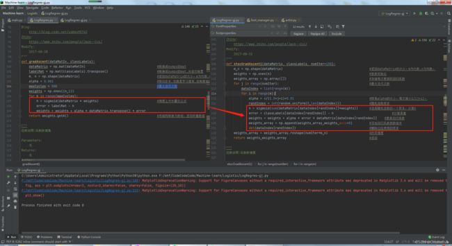
def stocGradAscent1(dataMatrix, classLabels, numIter=150):
    m,n = np.shape(dataMatrix)                                                #返回dataMatrix的大小。m为行数,n为列数。
    weights = np.ones(n)                                                       #参数初始化
    for j in range(numIter):
        dataIndex = list(range(m))
        for i in range(m):
            alpha = 4/(1.0+j+i)+0.01                                            #降低alpha的大小,每次减小1/(j+i)。
            randIndex = int(random.uniform(0,len(dataIndex)))                #随机选取样本
            h = sigmoid(sum(dataMatrix[randIndex]*weights))                    #选择随机选取的一个样本,计算h
            error = classLabels[randIndex] - h                                 #计算误差
            weights = weights + alpha * error * dataMatrix[randIndex]       #更新回归系数
            del(dataIndex[randIndex])                                         #删除已经使用的样本
    return weights                                                      #返回
完整代码如下:
# -*- coding:UTF-8 -*-
from matplotlib.font_manager import FontProperties
import matplotlib.pyplot as plt
import numpy as np
import random


"""
函数说明:加载数据

Parameters:
	无
Returns:
	dataMat - 数据列表
	labelMat - 标签列表
Author:
	Jack Cui
Blog:
	http://blog.csdn.net/c406495762
Zhihu:
	https://www.zhihu.com/people/Jack--Cui/
Modify:
	2017-08-28
"""
def loadDataSet():
	dataMat = []														#创建数据列表
	labelMat = []														#创建标签列表
	fr = open('testSet.txt')											#打开文件
	for line in fr.readlines():											#逐行读取
		lineArr = line.strip().split()									#去回车,放入列表
		dataMat.append([1.0, float(lineArr[0]), float(lineArr[1])])		#添加数据
		labelMat.append(int(lineArr[2]))								#添加标签
	fr.close()															#关闭文件
	return dataMat, labelMat											#返回

"""
函数说明:sigmoid函数

Parameters:
	inX - 数据
Returns:
	sigmoid函数
Author:
	Jack Cui
Blog:
	http://blog.csdn.net/c406495762
Zhihu:
	https://www.zhihu.com/people/Jack--Cui/
Modify:
	2017-08-28
"""
def sigmoid(inX):
	return 1.0 / (1 + np.exp(-inX))

"""
函数说明:梯度上升算法

Parameters:
	dataMatIn - 数据集
	classLabels - 数据标签
Returns:
	weights.getA() - 求得的权重数组(最优参数)
	weights_array - 每次更新的回归系数
Author:
	Jack Cui
Blog:
	http://blog.csdn.net/c406495762
Zhihu:
	https://www.zhihu.com/people/Jack--Cui/
Modify:
	2017-08-28
"""
def gradAscent(dataMatIn, classLabels):
	dataMatrix = np.mat(dataMatIn)										#转换成numpy的mat
	labelMat = np.mat(classLabels).transpose()							#转换成numpy的mat,并进行转置
	m, n = np.shape(dataMatrix)											#返回dataMatrix的大小。m为行数,n为列数。
	alpha = 0.01														#移动步长,也就是学习速率,控制更新的幅度。
	maxCycles = 500														#最大迭代次数
	weights = np.ones((n,1))
	weights_array = np.array([])
	for k in range(maxCycles):
		h = sigmoid(dataMatrix * weights)								#梯度上升矢量化公式
		error = labelMat - h
		weights = weights + alpha * dataMatrix.transpose() * error
		weights_array = np.append(weights_array,weights)
	weights_array = weights_array.reshape(maxCycles,n)
	return weights.getA(),weights_array									#将矩阵转换为数组,并返回

"""
函数说明:改进的随机梯度上升算法

Parameters:
	dataMatrix - 数据数组
	classLabels - 数据标签
	numIter - 迭代次数
Returns:
	weights - 求得的回归系数数组(最优参数)
	weights_array - 每次更新的回归系数
Author:
	Jack Cui
Blog:
	http://blog.csdn.net/c406495762
Zhihu:
	https://www.zhihu.com/people/Jack--Cui/
Modify:
	2017-08-31
"""
def stocGradAscent1(dataMatrix, classLabels, numIter=150):
	m,n = np.shape(dataMatrix)												#返回dataMatrix的大小。m为行数,n为列数。
	weights = np.ones(n)   													#参数初始化
	weights_array = np.array([])											#存储每次更新的回归系数
	for j in range(numIter):												#最大迭代次数
		dataIndex = list(range(m))
		for i in range(m):
			alpha = 4/(1.0+j+i)+0.01   	 									#降低alpha的大小,每次减小1/(j+i)。
			randIndex = int(random.uniform(0,len(dataIndex)))				#随机选取样本
			h = sigmoid(sum(dataMatrix[dataIndex[randIndex]]*weights))		#选择随机选取的一个样本,计算h
			error = classLabels[dataIndex[randIndex]] - h 								#计算误差
			weights = weights + alpha * error * dataMatrix[dataIndex[randIndex]]   	#更新回归系数
			weights_array = np.append(weights_array,weights,axis=0) 		#添加回归系数到数组中
			del(dataIndex[randIndex]) 										#删除已经使用的样本
	weights_array = weights_array.reshape(numIter*m,n) 						#改变维度
	return weights,weights_array 											#返回

"""
函数说明:绘制数据集

Parameters:
	weights - 权重参数数组
Returns:
	无
Author:
	Jack Cui
Blog:
	http://blog.csdn.net/c406495762
Zhihu:
	https://www.zhihu.com/people/Jack--Cui/
Modify:
	2017-08-30
"""
def plotBestFit(weights):
	dataMat, labelMat = loadDataSet()									#加载数据集
	dataArr = np.array(dataMat)											#转换成numpy的array数组
	n = np.shape(dataMat)[0]											#数据个数
	xcord1 = []; ycord1 = []											#正样本
	xcord2 = []; ycord2 = []											#负样本
	for i in range(n):													#根据数据集标签进行分类
		if int(labelMat[i]) == 1:
			xcord1.append(dataArr[i,1]); ycord1.append(dataArr[i,2])	#1为正样本
		else:
			xcord2.append(dataArr[i,1]); ycord2.append(dataArr[i,2])	#0为负样本
	fig = plt.figure()
	ax = fig.add_subplot(111)											#添加subplot
	ax.scatter(xcord1, ycord1, s = 20, c = 'red', marker = 's',alpha=.5)#绘制正样本
	ax.scatter(xcord2, ycord2, s = 20, c = 'green',alpha=.5)			#绘制负样本
	x = np.arange(-3.0, 3.0, 0.1)
	y = (-weights[0] - weights[1] * x) / weights[2]
	ax.plot(x, y)
	plt.title('BestFit')												#绘制title
	plt.xlabel('X1'); plt.ylabel('X2')									#绘制label
	plt.show()

"""
函数说明:绘制回归系数与迭代次数的关系

Parameters:
	weights_array1 - 回归系数数组1
	weights_array2 - 回归系数数组2
Returns:
	无
Author:
	Jack Cui
Blog:
	http://blog.csdn.net/c406495762
Zhihu:
	https://www.zhihu.com/people/Jack--Cui/
Modify:
	2017-08-30
"""
def plotWeights(weights_array1,weights_array2):
	#设置汉字格式
	font = FontProperties(fname=r"c:\windows\fonts\simsun.ttc", size=14)
	#将fig画布分隔成1行1列,不共享x轴和y轴,fig画布的大小为(13,8)
	#当nrow=3,nclos=2时,代表fig画布被分为六个区域,axs[0][0]表示第一行第一列
	fig, axs = plt.subplots(nrows=3, ncols=2,sharex=False, sharey=False, figsize=(20,10))
	x1 = np.arange(0, len(weights_array1), 1)
	#绘制w0与迭代次数的关系
	axs[0][0].plot(x1,weights_array1[:,0])
	axs0_title_text = axs[0][0].set_title(u'改进的随机梯度上升算法:回归系数与迭代次数关系',fontproperties=font)
	axs0_ylabel_text = axs[0][0].set_ylabel(u'W0',fontproperties=font)
	plt.setp(axs0_title_text, size=20, weight='bold', color='black')
	plt.setp(axs0_ylabel_text, size=20, weight='bold', color='black')
	#绘制w1与迭代次数的关系
	axs[1][0].plot(x1,weights_array1[:,1])
	axs1_ylabel_text = axs[1][0].set_ylabel(u'W1',fontproperties=font)
	plt.setp(axs1_ylabel_text, size=20, weight='bold', color='black')
	#绘制w2与迭代次数的关系
	axs[2][0].plot(x1,weights_array1[:,2])
	axs2_xlabel_text = axs[2][0].set_xlabel(u'迭代次数',fontproperties=font)
	axs2_ylabel_text = axs[2][0].set_ylabel(u'W1',fontproperties=font)
	plt.setp(axs2_xlabel_text, size=20, weight='bold', color='black')
	plt.setp(axs2_ylabel_text, size=20, weight='bold', color='black')


	x2 = np.arange(0, len(weights_array2), 1)
	#绘制w0与迭代次数的关系
	axs[0][1].plot(x2,weights_array2[:,0])
	axs0_title_text = axs[0][1].set_title(u'梯度上升算法:回归系数与迭代次数关系',fontproperties=font)
	axs0_ylabel_text = axs[0][1].set_ylabel(u'W0',fontproperties=font)
	plt.setp(axs0_title_text, size=20, weight='bold', color='black')
	plt.setp(axs0_ylabel_text, size=20, weight='bold', color='black')
	#绘制w1与迭代次数的关系
	axs[1][1].plot(x2,weights_array2[:,1])
	axs1_ylabel_text = axs[1][1].set_ylabel(u'W1',fontproperties=font)
	plt.setp(axs1_ylabel_text, size=20, weight='bold', color='black')
	#绘制w2与迭代次数的关系
	axs[2][1].plot(x2,weights_array2[:,2])
	axs2_xlabel_text = axs[2][1].set_xlabel(u'迭代次数',fontproperties=font)
	axs2_ylabel_text = axs[2][1].set_ylabel(u'W1',fontproperties=font)
	plt.setp(axs2_xlabel_text, size=20, weight='bold', color='black')
	plt.setp(axs2_ylabel_text, size=20, weight='bold', color='black')

	plt.show()

if __name__ == '__main__':
	dataMat, labelMat = loadDataSet()
	weights1,weights_array1 = stocGradAscent1(np.array(dataMat), labelMat)
	print(np.shape(weights_array1))
	print('weights1', weights1)
	print('weights_array1', weights_array1)
	# weights2,weights_array2 = gradAscent(dataMat, labelMat)
	# plotWeights(weights_array1, weights_array2)
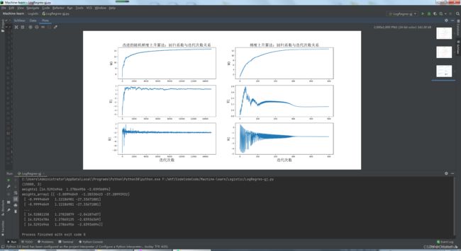
改进的随机梯度上升算法,在遍历数据集的第20次开始收敛。而梯度上升算法,在遍历数据集的第300次才开始收敛。
二、后续学习
2.1实战背景
本次实战内容,将使用Logistic回归来预测患疝气病的马的存活问题。原始数据集下载地址:这里的数据包含了368个样本和28个特征。这种病不一定源自马的肠胃问题,其他问题也可能引发马疝病。该数据集中包含了医院检测马疝病的一些指标,有的指标比较主观,有的指标难以测量,例如马的疼痛级别。另外需要说明的是,除了部分指标主观和难以测量外,该数据还存在一个问题,数据集中有30%的值是缺失的。下面将首先介绍如何处理数据集中的数据缺失问题,然后再利用Logistic回归和随机梯度上升算法来预测病马的生死。
2.2准备数据
我们常见的一些准备数据的方法有:
- 使用可用特征的均值来填补缺失值;
- 使用特殊值来填补缺失值,如-1;
- 忽略有缺失值的样本;
- 使用相似样本的均值添补缺失值;
- 使用另外的机器学习算法预测缺失值。
这里的数据集我们直接拿来用,是已经做过处理的数据集。
预处理数据做两件事:
- 如果测试集中一条数据的特征值已经确实,
那么我们选择实数0来替换所有缺失值,因为本文使用Logistic回归。因此这样做不会影响回归系数的值。sigmoid(0)=0.5,即它对结果的预测不具有任何倾向性。 - 如果测试集中一条数据的类别
标签已经缺失,那么我们将该类别数据丢弃,因为类别标签与特征不同,很难确定采用某个合适的值来替换。
2.3使用Python构建Logistic回归分类器
import numpy as np
import random

def sigmoid(inX):
    return 1.0 / (1 + np.exp(-inX))

def stocGradAscent1(dataMatrix, classLabels, numIter=150):
    m,n = np.shape(dataMatrix)                                                #返回dataMatrix的大小。m为行数,n为列数。
    weights = np.ones(n)                                                       #参数初始化                                        #存储每次更新的回归系数
    for j in range(numIter):
        dataIndex = list(range(m))
        for i in range(m):
            alpha = 4/(1.0+j+i)+0.01                                            #降低alpha的大小,每次减小1/(j+i)。
            randIndex = int(random.uniform(0,len(dataIndex)))                #随机选取样本
            h = sigmoid(sum(dataMatrix[randIndex]*weights))                    #选择随机选取的一个样本,计算h
            error = classLabels[randIndex] - h                                 #计算误差
            weights = weights + alpha * error * dataMatrix[randIndex]       #更新回归系数
            del(dataIndex[randIndex])                                         #删除已经使用的样本
    return weights                                                             #返回


def gradAscent(dataMatIn, classLabels):
    dataMatrix = np.mat(dataMatIn)                                        #转换成numpy的mat
    labelMat = np.mat(classLabels).transpose()                            #转换成numpy的mat,并进行转置
    m, n = np.shape(dataMatrix)                                            #返回dataMatrix的大小。m为行数,n为列数。
    alpha = 0.01                                                        #移动步长,也就是学习速率,控制更新的幅度。
    maxCycles = 500                                                        #最大迭代次数
    weights = np.ones((n,1))
    for k in range(maxCycles):
        h = sigmoid(dataMatrix * weights)                                #梯度上升矢量化公式
        error = labelMat - h
        weights = weights + alpha * dataMatrix.transpose() * error
    return weights.getA()                                                #将矩阵转换为数组,并返回

def classifyVector(inX, weights):
    prob = sigmoid(sum(inX * weights))
    if prob > 0.5:
        return 1.0
    else:
        return 0.0


def colicTest():
    # 数据处理
    frTrain = open('horseColicTraining.txt')
    frTest = open('horseColicTest.txt')
    trainingSet = []
    trainingLabels = []
    for line in frTrain.readlines():
        currline = line.strip().split(',')
        lineArr = []
        for i in range(len(currline) - 1):
            lineArr.append(float(currline[i]))
        trainingSet.append(lineArr)
        trainingLabels.append(float(currline[-1]))

    trainWeightsNew = stocGradAscent1(np.array(trainingSet), trainingLabels, 500)
    trainWeightsOld = gradAscent(trainingSet, trainingLabels)

    errorCountNew = 0
    errorCountOld = 0
    numTestVec = 0.0

    for line in frTest.readlines():
        numTestVec += 1.0
        currline = line.strip().split('\t')
        lineArr = []
        for i in range(len(currline) - 1):
            lineArr.append(float(currline[i]))

        # 这里注意符号
        if int((classifyVector(np.array(lineArr), trainWeightsNew))) != int(currline[-1]):
            errorCountNew += 1

        # 这里注意符号
        if int((classifyVector(np.array(lineArr), trainWeightsOld[:, 0]))) != int(currline[-1]):
            errorCountOld += 1


    errorRateNew = (float(errorCountNew) / numTestVec) * 100
    errorRateOld = (float(errorCountOld) / numTestVec) * 100

    print("随机测试集错误率为: %.2f%%\n" % errorRateNew)
    print("测试集错误率为: %.2f%%\n" % errorRateOld)


if __name__ == '__main__':
    colicTest()


随机测试集错误率为: 35.82%

测试集错误率为: 28.36%
结论:对比以后发现,随机梯度上升算法的错误率更高。大样本适合随机梯度上升算法,小样本还得是普通梯度上升算法。
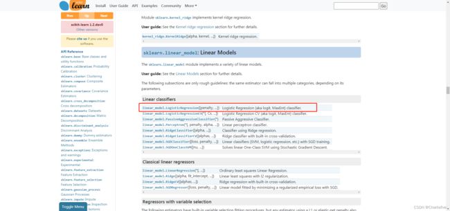
三、使用Sklearn构建Logistic回归分类器
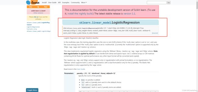
Sklearn的Logistic回归分类器官方英文文档地址:链接: https://scikit-learn.org/dev/modules/generated/sklearn.linear_model.LogisticRegression.html#sklearn.linear_model.LogisticRegression
参数描述请参考:链接: https://jackcui.blog.csdn.net/article/details/77851973
以及官方文档的链接: https://scikit-learn.org/dev/modules/generated/sklearn.linear_model.LogisticRegression.html#sklearn.linear_model.LogisticRegression
from sklearn.linear_model import LogisticRegression

def colicSklearn():
    # 数据处理
    frTrain = open('horseColicTraining.txt')
    frTest = open('horseColicTest.txt')
    trainingSet = []
    trainingLabels = []
    testSet = []
    testLabels = []

    for line in frTrain.readlines():
        currline = line.strip().split(',')
        lineArr = []
        for i in range(len(currline) - 1):
            lineArr.append(float(currline[i]))
        trainingSet.append(lineArr)
        trainingLabels.append(float(currline[-1]))

    for line in frTest.readlines():
        currline = line.strip().split('\t')
        lineArr = []
        for i in range(len(currline) - 1):
            lineArr.append(float(currline[i]))
        testSet.append(lineArr)
        testLabels.append(float(currline[-1]))

    classifier = LogisticRegression(solver='liblinear', max_iter=10).fit(trainingSet, trainingLabels)
    classifier2 = LogisticRegression(solver='sag', max_iter=5000).fit(trainingSet, trainingLabels)
    test_accurcy = classifier.score(testSet, testLabels) * 100
    test_accurcy2 = classifier2.score(testSet, testLabels) * 100

    print('正确率:%f%%' % test_accurcy)
    print('随机梯度下降正确率:%f%%' % test_accurcy2)

if __name__ == '__main__':
    colicSklearn()


ConvergenceWarning: Liblinear failed to converge, increase the number of iterations.
  warnings.warn(
正确率:73.134328%
随机梯度下降正确率:73.134328%

Process finished with exit code 0
可以看到,对于我们这样的小数据集,sag算法需要迭代上千次才收敛,而liblinear只需要不到10次。
还是那句话,我们需要根据数据集情况,选择最优化算法。
四、总结
1 Logistic回归的优缺点
优点:
实现简单,易于理解和实现;计算代价不高,速度很快,存储资源低。
缺点:
容易欠拟合,分类精度可能不高。
2 其他
Logistic回归的目的是寻找一个非线性函数Sigmoid的最佳拟合参数,求解过程可以由最优化算法完成。
改进的一些最优化算法,比如sag。它可以在新数据到来时就完成参数更新,而不需要重新读取整个数据集来进行批量处理。
机器学习的一个重要问题就是如何处理缺失数据。这个问题没有标准答案,取决于实际应用中的需求。现有一些解决方案,每种方案都各有优缺点。
我们需要根据数据的情况,这是Sklearn的参数,以期达到更好的分类效果。