机器学习实战（二）：End-to-End Machine Learning Project

房地产项目步骤：

• Look at the big picture.（观察大局）
• Get the data.
• Discover and visualize the data to gain insights.（从数据探索和可视化得到东健）
• Prepare the data for Machine Learning algorithms.
• Select a model and train it.
• Fine-tune your model.（微调模型）
• Present your solution.
• Launch, monitor, and maintain your system.（启动、监控和维护系统）

Look at the Big Picture

需要从数据中学习，根据所有其他指标，预测任意区域房价中位数

Frame the Problem

机器学习流水线（Pipelines）
是否是监督式？给出了所有标记的训练实例（每个实例都有预期产出：房价中位数），典型的监督式。
是回归、分类还是其他任务？典型回归任务，需要对某个值进行预测（多变量回归问题）
批量还是在线？批量，因为数据集不大，也没有持续流入系统。

Select a Performance Measure（选择性能指标）

回归问题典型性能指标：

• 均方根误差（Root Mean Square Error (RMSE)）
• 平均绝对误差（ Mean Absolute Error（MAE）
  范数指数越高越关注大的价值，RMSE比MAE更敏感，异常值少时更优异

Check the Assumptions（检查假设）

确定任务类型

Get the Data

Create the Workspace （创建工作区）

使用 Jupyter Notebook运行。（命令行 虚拟环境不予展示，windows版本不同，用Anaconda）

做一些准备

引库，画图，保存（目前没啥用）

from __future__ import division, print_function, unicode_literals

# Common imports
import numpy as np
import os

# to make this notebook's output stable across runs
np.random.seed(42)

# To plot pretty figures
%matplotlib inline
import matplotlib as mpl
import matplotlib.pyplot as plt
mpl.rc('axes', labelsize=14)
mpl.rc('xtick', labelsize=12)
mpl.rc('ytick', labelsize=12)

# Where to save the figures
PROJECT_ROOT_DIR = "."
CHAPTER_ID = "end_to_end_project"
IMAGES_PATH = os.path.join(PROJECT_ROOT_DIR, "images", CHAPTER_ID)

def save_fig(fig_id, tight_layout=True, fig_extension="png", resolution=300):
    path = os.path.join(IMAGES_PATH, fig_id + "." + fig_extension)
    print("Saving figure", fig_id)
    if tight_layout:
        plt.tight_layout()
    plt.savefig(path, format=fig_extension, dpi=resolution)

# Ignore useless warnings (see SciPy issue #5998)
import warnings
warnings.filterwarnings(action="ignore", message="^internal gelsd")

Download the Data

有些批注在jupyter notebook里，此处直接CV了，调用fetch_housing_data时，自动创建目录下载解压文件。

import os
import tarfile
from six.moves import urllib

DOWNLOAD_ROOT = "https://raw.githubusercontent.com/ageron/handson-ml/master/"
HOUSING_PATH = os.path.join("datasets", "housing")
HOUSING_URL = DOWNLOAD_ROOT + "datasets/housing/housing.tgz"

def fetch_housing_data(housing_url=HOUSING_URL, housing_path=HOUSING_PATH):
    os.makedirs(housing_path, exist_ok=True)
    tgz_path = os.path.join(housing_path, "housing.tgz")
    urllib.request.urlretrieve(housing_url, tgz_path)
    housing_tgz = tarfile.open(tgz_path)
    housing_tgz.extractall(path=housing_path)
    housing_tgz.close()

用Pandas加载数据（关于Pandas也是需要入门学习的），返回一个 Pandas DataFrame对象。

Take a Quick Look at the Data Structure

DataFrames和head()方法可以查看前五行；使用info()方法可以获取数据集简单描述（总行数、每个属性类型，非空值数量）；使用某属性的value_counts()方法可以查看多少种分类存在及所辖区域个数，例如housing["ocean_proximity"].value_counts()；用describe()可以查看数值属性摘要，如（count、max、min、mean，std（标准差））

绘制直方图也可，调用hist()方法

%matplotlib inline
import matplotlib.pyplot as plt
housing.hist(bins=50, figsize=(20,15))
plt.show()

Matplotlib的使用，一般用jupyter 的%matplotlib inline命令

创建测试集

使用函数创建：

from sklearn.model_selection import train_test_split
train_set, test_set = train_test_split(housing, test_size=0.2, random_state=42)

查看中位数housing["median_income"].hist()
创建收入类别属性：中位数/1.5（限制收入类别数量），使用ceil取整（得到离散类别），再大的合并到类别5：

housing["income_cat"] = np.ceil(housing["median_income"] / 1.5)
housing["income_cat"].where(housing["income_cat"] < 5, 5.0, inplace=True)

使用 Scikit-Learn的 StratifiedShuffleSplit类抽样：

from sklearn.model_selection import StratifiedShuffleSplit

split = StratifiedShuffleSplit(n_splits=1, test_size=0.2, random_state=42)
for train_index, test_index in split.split(housing, housing["income_cat"]):
    strat_train_set = housing.loc[train_index]
    strat_test_set = housing.loc[test_index]

查看住房根据收入比例housing["income_cat"].value_counts() / len(housing)
查看其他数据集收入类别比例（完整数据集、分层抽样数据集、纯随机抽样数据集）（见jupyter）
删除income_cat属性

for set_ in (strat_train_set, strat_test_set):
    set_.drop("income_cat", axis=1, inplace=True)

Discover and Visualize the Data to Gain Insights

创建副本housing = strat_train_set.copy()
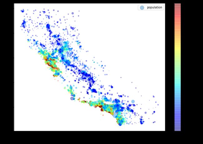
根据经纬度，密度（alpha），人口数量，预订颜色表（jet）可视化

housing.plot(kind="scatter", x="longitude", y="latitude", alpha=0.4,
    s=housing["population"]/100, label="population", figsize=(10,7),
    c="median_house_value", cmap=plt.get_cmap("jet"), colorbar=True,
    sharex=False)
plt.legend()

Looking for Correlations（寻找相关性）

数据集不大，直接用corr()方法计算standard correlation coeffcient (also called Pearson’s r)标准相关系数，也叫皮埃尔系数：corr_matrix = housing.corr()
想看看每个属性与房屋中位数相关性corr_matrix["median_house_value"].sort_values(ascending=False)
1：正相关，-1：负相关，0：无关

利用Pandas的scatter_matrix函数绘制：

# from pandas.tools.plotting import scatter_matrix # For older versions of Pandas
from pandas.plotting import scatter_matrix

attributes = ["median_house_value", "median_income", "total_rooms",
              "housing_median_age"]
scatter_matrix(housing[attributes], figsize=(12, 8))

显然为收入中位数，放大查看相关性：housing.plot(kind="scatter", x="median_income",y="median_house_value",alpha=0.1)
有怪异的直线，可以尝试删除

Experimenting with Attribute Combinations（尝试不同属性结合）

房间总数，卧室总数，总人数对于房屋均价意义不大，创造新属性人均持有量更有意义。

housing["rooms_per_household"] = housing["total_rooms"]/housing["households"]
housing["bedrooms_per_room"] = housing["total_bedrooms"]/housing["total_rooms"]
housing["population_per_household"]=housing["population"]/housing["households"]

查看关联矩阵

housing.plot(kind="scatter", x="rooms_per_household", y="median_house_value",
             alpha=0.2)
plt.axis([0, 5, 0, 520000])
plt.show()

badromes_per_rome相关性高很多

Prepare the Data for Machine Learning Algorithms

Data Cleaning

大部分机器学习算法无法在缺失特征上工作，所以需要创建函数，方法

• 放弃相应地区（dropna()）
• 放弃这个属性（drop()）
• 将缺失值设为特定值（0,mean,median and so on）

median = housing["total_bedrooms"].median()
sample_incomplete_rows["total_bedrooms"].fillna(median, inplace=True) # option 3

Scikit-Learn提供了imputer来处理缺失值：
创建imputer实例

try:
    from sklearn.impute import SimpleImputer # Scikit-Learn 0.20+
except ImportError:
    from sklearn.preprocessing import Imputer as SimpleImputer
imputer = SimpleImputer(strategy="median")

中位数只能在没有文本属性的数值上运算，创建副本housing_num = housing.drop('ocean_proximity', axis=1)
fit()适配：imputer.fit(housing_num)
稳妥起见应用到所有数值属性：

imputer.statistics_
housing_num.median().values

使用imputer将缺失值替换为中位数完成训练集替换X = imputer.transform(housing_num)
将Numpy数组放回 Pandas DataFramehousing_tr = pd.DataFrame(X, columns=housing_num.columns, index=housing.index)

Scikit-Learn设计原则（具体表述见书）

• Consistency（一致性）：Estimators（估算器）、Transformers（转换器）、Predictors（预测器）
• Inspection
• Nonproliferation of classes.（放置类扩散）
• Composition（构成）
• Sensible defaults（合力默认值）

Handling Text and Categorical Attributes（处理文本属性）

Scikit-Learn提供 OrdinalEncoder转换文字属性

try:
    from sklearn.preprocessing import OrdinalEncoder
except ImportError:
    from future_encoders import OrdinalEncoder # Scikit-Learn < 0.20
    
ordinal_encoder = OrdinalEncoder()
housing_cat_encoded = ordinal_encoder.fit_transform(housing_cat)
housing_cat_encoded[:10]

独热编码：0,4比0,1相似度更高，所以只有一个属性为热1，其余均为冷0
Scikit-Learn提供OneHotEncoder编码，将整数分类转换为独热向量（OrdinalEncoder将housing_cat_encoded 转换为二维数组），得到的是系数矩阵，如果想稠密调用toarray()。

Custom Transformers（自定义转换器）

创建一个类，使用fit()（返回自身）、tansform()、fit_transform(),使用BaseEstimator做基类得到get_params()、set_params()方法，使用TransformerMixin做基类直接得到最后一种方法。

from sklearn.base import BaseEstimator, TransformerMixin

# get the right column indices: safer than hard-coding indices 3, 4, 5, 6
rooms_ix, bedrooms_ix, population_ix, household_ix = [
    list(housing.columns).index(col)
    for col in ("total_rooms", "total_bedrooms", "population", "households")]

class CombinedAttributesAdder(BaseEstimator, TransformerMixin):
    def __init__(self, add_bedrooms_per_room = True): # no *args or **kwargs 是否有助于机器学习算法
        self.add_bedrooms_per_room = add_bedrooms_per_room
    def fit(self, X, y=None):
        return self  # nothing else to do
    def transform(self, X, y=None):
        rooms_per_household = X[:, rooms_ix] / X[:, household_ix]
        population_per_household = X[:, population_ix] / X[:, household_ix]
        if self.add_bedrooms_per_room:
            bedrooms_per_room = X[:, bedrooms_ix] / X[:, rooms_ix]
            return np.c_[X, rooms_per_household, population_per_household,
                         bedrooms_per_room]
        else:
            return np.c_[X, rooms_per_household, population_per_household]

attr_adder = CombinedAttributesAdder(add_bedrooms_per_room=False)
housing_extra_attribs = attr_adder.transform(housing.values)

Feature Scaling（特征缩放）

大小相差太大可能会使机器学习算法表现不佳。
Min-max scaling（最大最小缩放）/normalization（归一化）：缩放使归于0-1——（value - min）/（max-min）,Scikit-Learn提供MinMaxScaler转换器，可通过调整超参数feature_range修改范围
Standardization（标准化）：（value - mean）/variance（方差）受异常值影响小。Scikit-Learn提供StandardScaler转换器。

Transformation Pipelines

数据转换步骤按正确顺序执行，数值型流水线实例：

from sklearn.pipeline import Pipeline
from sklearn.preprocessing import StandardScaler

num_pipeline = Pipeline([
        ('imputer', SimpleImputer(strategy="median")),
        ('attribs_adder', FunctionTransformer(add_extra_features, validate=False)),
        ('std_scaler', StandardScaler()),
    ])

housing_num_tr = num_pipeline.fit_transform(housing_num)

Scikit-Learn提供ColumnTransformer来构造：

try:
    from sklearn.compose import ColumnTransformer
except ImportError:
    from future_encoders import ColumnTransformer # Scikit-Learn < 0.20
    
num_attribs = list(housing_num)
cat_attribs = ["ocean_proximity"]

full_pipeline = ColumnTransformer([
        ("num", num_pipeline, num_attribs),
        ("cat", OneHotEncoder(), cat_attribs),
    ])

housing_prepared = full_pipeline.fit_transform(housing)

Select and Train a Model

Training and Evaluating on the Training Set

先训练一个线性回归模型：

 
from sklearn.linear_model import LinearRegression

lin_reg = LinearRegression()
lin_reg.fit(housing_prepared, housing_labels)

训练几个实例试试

some_data = housing.iloc[:5]#前闭后开
some_labels = housing_labels.iloc[:5]
some_data_prepared = full_pipeline.transform(some_data)# 调用full_pipeline对数据进行预处理
print("Predictions:", lin_reg.predict(some_data_prepared))
print("Labels:", list(some_labels))

使用mean_squared_error测量回归模型RMSE。

from sklearn.metrics import mean_squared_error

housing_predictions = lin_reg.predict(housing_prepared)
lin_mse = mean_squared_error(housing_labels, housing_predictions)
lin_rmse = np.sqrt(lin_mse)
lin_rmse

训练一个DecisionTreeRegressor

from sklearn.tree import DecisionTreeRegressor

tree_reg = DecisionTreeRegressor(random_state=42)
tree_reg.fit(housing_prepared, housing_labels)

评估一下

housing_predictions = tree_reg.predict(housing_prepared)
tree_mse = mean_squared_error(housing_labels, housing_predictions)
tree_rmse = np.sqrt(tree_mse)
tree_rmse

Better Evaluation Using Cross-Validation

执行 cross-validation feature，折叠评估

from sklearn.model_selection import cross_val_score

scores = cross_val_score(tree_reg, housing_prepared, housing_labels,
                         scoring="neg_mean_squared_error", cv=10)
tree_rmse_scores = np.sqrt(-scores)

查看结果

def display_scores(scores):
    print("Scores:", scores)
    print("Mean:", scores.mean())
    print("Standard deviation:", scores.std())

display_scores(tree_rmse_scores)

看一下线性回归

lin_scores = cross_val_score(lin_reg, housing_prepared, housing_labels,
                             scoring="neg_mean_squared_error", cv=10)
lin_rmse_scores = np.sqrt(-lin_scores)
display_scores(lin_rmse_scores)

试一下最后一个模型，随机森林，继承学习，多个决策树取平均：

from sklearn.ensemble import RandomForestRegressor

forest_reg = RandomForestRegressor(n_estimators=10, random_state=42)
forest_reg.fit(housing_prepared, housing_labels)


housing_predictions = forest_reg.predict(housing_prepared)
forest_mse = mean_squared_error(housing_labels, housing_predictions)
forest_rmse = np.sqrt(forest_mse)
forest_rmse

from sklearn.model_selection import cross_val_score

forest_scores = cross_val_score(forest_reg, housing_prepared, housing_labels,
                                scoring="neg_mean_squared_error", cv=10)
forest_rmse_scores = np.sqrt(-forest_scores)
display_scores(forest_rmse_scores)

通过sklearn.externals.joblib保存模型（再探讨）。

Fine-Tune Your Model（微调模型）

Grid Search网格搜索

使用Scikit-Learn的GridSearchCV微调模型，基于超参数与尝试值，它使用交叉验证得到最佳组合

from sklearn.model_selection import GridSearchCV

param_grid = [
    # try 12 (3×4) combinations of hyperparameters
    {'n_estimators': [3, 10, 30], 'max_features': [2, 4, 6, 8]},
    # then try 6 (2×3) combinations with bootstrap set as False
    {'bootstrap': [False], 'n_estimators': [3, 10], 'max_features': [2, 3, 4]},
  ]

forest_reg = RandomForestRegressor(random_state=42)
# train across 5 folds, that's a total of (12+6)*5=90 rounds of training 
grid_search = GridSearchCV(forest_reg, param_grid, cv=5,

                           scoring='neg_mean_squared_error', return_train_score=True)
grid_search.fit(housing_prepared, housing_labels)

得到最佳参数组合：grid_search.best_params_
得到最好的估算器：grid_search.best_estimator_

Randomized Search（随机搜索）

RandomizedSearchCV
数据集较大优先，随机搜索多少个迭代，搜索每个超参数多少不同的值。可控制计算预算

from sklearn.model_selection import RandomizedSearchCV
from scipy.stats import randint

param_distribs = {
        'n_estimators': randint(low=1, high=200),
        'max_features': randint(low=1, high=8),
    }

forest_reg = RandomForestRegressor(random_state=42)
rnd_search = RandomizedSearchCV(forest_reg, param_distributions=param_distribs,
                                n_iter=10, cv=5, scoring='neg_mean_squared_error', random_state=42)
rnd_search.fit(housing_prepared, housing_labels)

Ensemble Methods（集成方法)

将最优模型组合（charter7）

Analyze the Best Models and Their Errors

RandomForestRegressor可给予每个属性重要程度，将分数显示在对应属性旁：

feature_importances = grid_search.best_estimator_.feature_importances_
extra_attribs = ["rooms_per_hhold", "pop_per_hhold", "bedrooms_per_room"]
#cat_encoder = cat_pipeline.named_steps["cat_encoder"] # old solution
cat_encoder = full_pipeline.named_transformers_["cat"]
cat_one_hot_attribs = list(cat_encoder.categories_[0])
attributes = num_attribs + extra_attribs + cat_one_hot_attribs
sorted(zip(feature_importances, attributes), reverse=True)

尝试删除不太有用特征。

Evaluate Your System on the Test Set

运行full_pipeline转换（调用transform（））

final_model = grid_search.best_estimator_

X_test = strat_test_set.drop("median_house_value", axis=1)
y_test = strat_test_set["median_house_value"].copy()

X_test_prepared = full_pipeline.transform(X_test)
final_predictions = final_model.predict(X_test_prepared)

final_mse = mean_squared_error(y_test, final_predictions)
final_rmse = np.sqrt(final_mse)

Launch, Monitor, and Maintain Your System