深度学习(二)——经典网络LeNet+Pytorch实现

LeNet神经网络介绍

LeNet神经网络由深度学习三巨头之一的Yan LeCun提出，他同时也是卷积神经网络 (CNN，Convolutional Neural Networks)之父。LeNet主要用来进行手写字符的识别与分类，并在美国的银行中投入了使用。LeNet的实现确立了CNN的结构，现在神经网络中的许多内容在LeNet的网络结构中都能看到，例如卷积层，Pooling层，ReLU层。虽然LeNet早在20世纪90年代就已经提出了，但由于当时缺乏大规模的训练数据，计算机硬件的性能也较低，因此LeNet神经网络在处理复杂问题时效果并不理想。虽然LeNet网络结构比较简单，但是刚好适合神经网络的入门学习。

---

LeNet神经网络结构

LeNet的神经网络结构图如下：

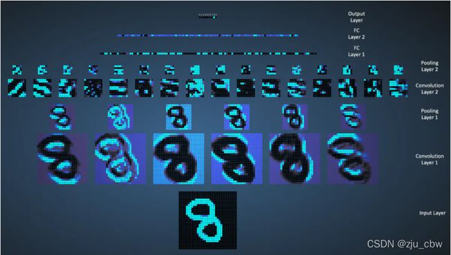
LeNet网络的执行流程图如下：

LeNet各层的参数变化

• C1
  输入大小：32*32
  核大小：5*5
  核数目：6
  输出大小：28*28*6
  训练参数数目：(5*5+1)*6=156
  连接数：(5*5+1)*6*(32-2-2)*(32-2-2)=122304

• S2
  输入大小：28*28*6
  核大小：2*2
  核数目：1
  输出大小：14*14*6
  训练参数数目：2*6=12，2=(w,b)
  连接数：(2*2+1)*1*14*14*6 = 5880

• C3
  输入大小：14*14*6
  核大小：5*5
  核数目：16
  输出大小：10*10*16
  训练参数数目：6*(3*5*5+1) + 6*(4*5*5+1) + 3*(4*5*5+1) + 1*(6*5*5+1)=1516
  连接数：(6*(3*5*5+1) + 6*(4*5*5+1) + 3*(4*5*5+1) + 1*(6*5*5+1))*10*10=151600

• S4
  输入大小：10*10*16
  核大小：2*2
  核数目：1
  输出大小：5*5*16
  训练参数数目：2*16=32
  连接数：(2*2+1)*1*5*5*16=2000

• C5
  输入大小：5*5*16
  核大小：5*5
  核数目：120
  输出大小：120*1*1
  训练参数数目：(5*5*16+1)*120*1*1=48120（因为是全连接）
  连接数：(5*5*16+1)*120*1*1=48120

• F6
  输入大小：120
  输出大小：84
  训练参数数目：(120+1)*84=10164
  连接数：(120+1)*84=10164

LeNet第三层（卷积操作）

值得关注的是LeNet第三层，LeNet第三层（C3层）也是卷积层，卷积核大小仍为5*5，不过卷积核的数量变为16个。第三层的输入为14*14的6个feature map，卷积核大小为5*5，因此卷积之后输出的feature map大小为10*10，由于卷积核有16个，因此希望输出的feature map也为16个，但由于输入有6个feature map，因此需要进行额外的处理。输入的6个feature map与输出的16个feature map的关系图如下：

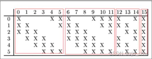
如上图所示，第一个卷积核处理前三幅输入的feature map，得出一个新的feature map。

---

LetNet(Pytorch版本)

model.py

import torch.nn as nn
import torch.nn.functional as F

class LeNet(nn.Module):
    def __init__(self):
        super(LeNet,self).__init__()
        self.conv1 = nn.Conv2d(3,16,5)
        self.pool1 = nn.MaxPool2d(2,2)
        self.conv2 = nn.Conv2d(16,32,5)
        self.pool2 = nn.MaxPool2d(2,2)
        self.fc1 = nn.Linear(32*5*5,120)
        self.fc2 = nn.Linear(120,84)
        self.fc3 = nn.Linear(84,10)
    
    def forward(self, x):
        x = F.relu(self.conv1(x))#input(3,32,32) output(16,28,28)
        x = self.pool1(x) #output(16，14，14)
        x = F.relu(self.conv2(x)) #output(32,10.10)
        x = self.pool2(x) #output(32,5,5)
        x = x.view(-1,32*5*5) #output(5*5*32)
        x = F.relu(self.fc1(x)) #output(120)
        x = F.relu(self.fc2(x)) #output(84)
        x = self.fc3(x) #output(10)
        return x

#model调试
import torch

#定义shape
input1 = torch.rand([32,3,32,32])
model = LeNet()#实例化
print(model)
#输入网络中
output = model(input1)

train.py

#train.py

import torch
import torchvision
import torch.nn as nn
import torch.optim as optim
import torchvision.transforms as transforms
from torchvision import transforms, datasets, utils
import matplotlib.pyplot as plt
import numpy as np


#device : GPU or CPU
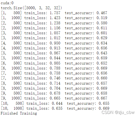
device = torch.device("cuda:0" if torch.cuda.is_available() else "cpu")
print(device)


transform = transforms.Compose(
    [transforms.ToTensor(),
     transforms.Normalize((0.5, 0.5, 0.5), (0.5, 0.5, 0.5))])

# 50000张训练图片
train_set = torchvision.datasets.CIFAR10(root='./data', train=True,
                                         download=False, transform=transform)
train_loader = torch.utils.data.DataLoader(train_set, batch_size=36,
                                           shuffle=False, num_workers=0)

# 10000张验证图片
val_set = torchvision.datasets.CIFAR10(root='./data', train=False,
                                       download=False, transform=transform)
val_loader = torch.utils.data.DataLoader(val_set, batch_size=5000,
                                         shuffle=False, num_workers=0)
val_data_iter = iter(val_loader)
val_image, val_label = val_data_iter.next()
print(val_image.size())
# print(train_set.class_to_idx)
# classes = ('plane', 'car', 'bird', 'cat',
#           'deer', 'dog', 'frog', 'horse', 'ship', 'truck')
#
#
# #显示图像，之前需把validate_loader中batch_size改为4
# aaa = train_set.class_to_idx
# cla_dict = dict((val, key) for key, val in aaa.items())
# def imshow(img):
#     img = img / 2 + 0.5  # unnormalize
#     npimg = img.numpy()
#     plt.imshow(np.transpose(npimg, (1, 2, 0)))
#     plt.show()
#
# print(' '.join('%5s' % cla_dict[val_label[j].item()] for j in range(4)))
# imshow(utils.make_grid(val_image))




net = LeNet()
net.to(device)

loss_function = nn.CrossEntropyLoss()
#定义优化器
optimizer = optim.Adam(net.parameters(), lr=0.001)

#训练过程
for epoch in range(10):  # loop over the dataset multiple times

    running_loss = 0.0 #累加损失
    for step, data in enumerate(train_loader, start=0):
        # get the inputs; data is a list of [inputs, labels]
        inputs, labels = data
        #print(inputs.size(), labels.size())
        # zero the parameter gradients
        optimizer.zero_grad()#如果不清除历史梯度，就会对计算的历史梯度进行累加
        # forward + backward + optimize
        outputs = net(inputs.to(device))
        loss = loss_function(outputs, labels.to(device))
        loss.backward()
        optimizer.step()

        # print statistics
        running_loss += loss.item()
        if step % 500 == 499:    # print every 500 mini-batches
            with torch.no_grad():#上下文管理器
                outputs = net(val_image.to(device))  # [batch, 10]
                predict_y = torch.max(outputs, dim=1)[1]
                accuracy = (predict_y == val_label.to(device)).sum().item() / val_label.size(0)

                print('[%d, %5d] train_loss: %.3f  test_accuracy: %.3f' %
                      (epoch + 1, step + 1, running_loss / 500, accuracy))
                running_loss = 0.0

print('Finished Training')

save_path = './Lenet.pth'
torch.save(net.state_dict(), save_path)