机器学习-聚类算法-01

机器学习-聚类算法-01
机器学习-聚类算法-02

K-Means算法

1. 理论基础

• k-means算法属于无监督学习算法

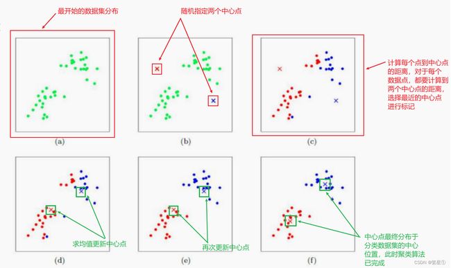
• 核心步骤有两点：

  1. 距离的计算
  2. 中心点的更新

• 基本概念：

  • 簇：就是分类的数量，需要指定
  • 质心：均值，就是向量各维取平均
  • 距离的度量：常用欧几里得距离和余弦相似度
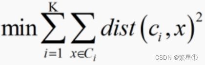
  • 优化目标：

• 工作流程
  

• 优点：

  简单，快速，适合常规数据集

• 缺点：

  1. K值难确定
  2. 复杂度与样本呈线性关系
  3. 很难发现任意形状的簇
     

2. 具体代码

2.1. 数据集

(iris.csv)

sepal_length,sepal_width,petal_length,petal_width,class
5.1,3.5,1.4,0.2,SETOSA
4.9,3.0,1.4,0.2,SETOSA
4.7,3.2,1.3,0.2,SETOSA
4.6,3.1,1.5,0.2,SETOSA
5.0,3.6,1.4,0.2,SETOSA
5.4,3.9,1.7,0.4,SETOSA
4.6,3.4,1.4,0.3,SETOSA
5.0,3.4,1.5,0.2,SETOSA
4.4,2.9,1.4,0.2,SETOSA
4.9,3.1,1.5,0.1,SETOSA
5.4,3.7,1.5,0.2,SETOSA
4.8,3.4,1.6,0.2,SETOSA
4.8,3.0,1.4,0.1,SETOSA
4.3,3.0,1.1,0.1,SETOSA
5.8,4.0,1.2,0.2,SETOSA
5.7,4.4,1.5,0.4,SETOSA
5.4,3.9,1.3,0.4,SETOSA
5.1,3.5,1.4,0.3,SETOSA
5.7,3.8,1.7,0.3,SETOSA
5.1,3.8,1.5,0.3,SETOSA
5.4,3.4,1.7,0.2,SETOSA
5.1,3.7,1.5,0.4,SETOSA
4.6,3.6,1.0,0.2,SETOSA
5.1,3.3,1.7,0.5,SETOSA
4.8,3.4,1.9,0.2,SETOSA
5.0,3.0,1.6,0.2,SETOSA
5.0,3.4,1.6,0.4,SETOSA
5.2,3.5,1.5,0.2,SETOSA
5.2,3.4,1.4,0.2,SETOSA
4.7,3.2,1.6,0.2,SETOSA
4.8,3.1,1.6,0.2,SETOSA
5.4,3.4,1.5,0.4,SETOSA
5.2,4.1,1.5,0.1,SETOSA
5.5,4.2,1.4,0.2,SETOSA
4.9,3.1,1.5,0.1,SETOSA
5.0,3.2,1.2,0.2,SETOSA
5.5,3.5,1.3,0.2,SETOSA
4.9,3.1,1.5,0.1,SETOSA
4.4,3.0,1.3,0.2,SETOSA
5.1,3.4,1.5,0.2,SETOSA
5.0,3.5,1.3,0.3,SETOSA
4.5,2.3,1.3,0.3,SETOSA
4.4,3.2,1.3,0.2,SETOSA
5.0,3.5,1.6,0.6,SETOSA
5.1,3.8,1.9,0.4,SETOSA
4.8,3.0,1.4,0.3,SETOSA
5.1,3.8,1.6,0.2,SETOSA
4.6,3.2,1.4,0.2,SETOSA
5.3,3.7,1.5,0.2,SETOSA
5.0,3.3,1.4,0.2,SETOSA
7.0,3.2,4.7,1.4,VERSICOLOR
6.4,3.2,4.5,1.5,VERSICOLOR
6.9,3.1,4.9,1.5,VERSICOLOR
5.5,2.3,4.0,1.3,VERSICOLOR
6.5,2.8,4.6,1.5,VERSICOLOR
5.7,2.8,4.5,1.3,VERSICOLOR
6.3,3.3,4.7,1.6,VERSICOLOR
4.9,2.4,3.3,1.0,VERSICOLOR
6.6,2.9,4.6,1.3,VERSICOLOR
5.2,2.7,3.9,1.4,VERSICOLOR
5.0,2.0,3.5,1.0,VERSICOLOR
5.9,3.0,4.2,1.5,VERSICOLOR
6.0,2.2,4.0,1.0,VERSICOLOR
6.1,2.9,4.7,1.4,VERSICOLOR
5.6,2.9,3.6,1.3,VERSICOLOR
6.7,3.1,4.4,1.4,VERSICOLOR
5.6,3.0,4.5,1.5,VERSICOLOR
5.8,2.7,4.1,1.0,VERSICOLOR
6.2,2.2,4.5,1.5,VERSICOLOR
5.6,2.5,3.9,1.1,VERSICOLOR
5.9,3.2,4.8,1.8,VERSICOLOR
6.1,2.8,4.0,1.3,VERSICOLOR
6.3,2.5,4.9,1.5,VERSICOLOR
6.1,2.8,4.7,1.2,VERSICOLOR
6.4,2.9,4.3,1.3,VERSICOLOR
6.6,3.0,4.4,1.4,VERSICOLOR
6.8,2.8,4.8,1.4,VERSICOLOR
6.7,3.0,5.0,1.7,VERSICOLOR
6.0,2.9,4.5,1.5,VERSICOLOR
5.7,2.6,3.5,1.0,VERSICOLOR
5.5,2.4,3.8,1.1,VERSICOLOR
5.5,2.4,3.7,1.0,VERSICOLOR
5.8,2.7,3.9,1.2,VERSICOLOR
6.0,2.7,5.1,1.6,VERSICOLOR
5.4,3.0,4.5,1.5,VERSICOLOR
6.0,3.4,4.5,1.6,VERSICOLOR
6.7,3.1,4.7,1.5,VERSICOLOR
6.3,2.3,4.4,1.3,VERSICOLOR
5.6,3.0,4.1,1.3,VERSICOLOR
5.5,2.5,4.0,1.3,VERSICOLOR
5.5,2.6,4.4,1.2,VERSICOLOR
6.1,3.0,4.6,1.4,VERSICOLOR
5.8,2.6,4.0,1.2,VERSICOLOR
5.0,2.3,3.3,1.0,VERSICOLOR
5.6,2.7,4.2,1.3,VERSICOLOR
5.7,3.0,4.2,1.2,VERSICOLOR
5.7,2.9,4.2,1.3,VERSICOLOR
6.2,2.9,4.3,1.3,VERSICOLOR
5.1,2.5,3.0,1.1,VERSICOLOR
5.7,2.8,4.1,1.3,VERSICOLOR
6.3,3.3,6.0,2.5,VIRGINICA
5.8,2.7,5.1,1.9,VIRGINICA
7.1,3.0,5.9,2.1,VIRGINICA
6.3,2.9,5.6,1.8,VIRGINICA
6.5,3.0,5.8,2.2,VIRGINICA
7.6,3.0,6.6,2.1,VIRGINICA
4.9,2.5,4.5,1.7,VIRGINICA
7.3,2.9,6.3,1.8,VIRGINICA
6.7,2.5,5.8,1.8,VIRGINICA
7.2,3.6,6.1,2.5,VIRGINICA
6.5,3.2,5.1,2.0,VIRGINICA
6.4,2.7,5.3,1.9,VIRGINICA
6.8,3.0,5.5,2.1,VIRGINICA
5.7,2.5,5.0,2.0,VIRGINICA
5.8,2.8,5.1,2.4,VIRGINICA
6.4,3.2,5.3,2.3,VIRGINICA
6.5,3.0,5.5,1.8,VIRGINICA
7.7,3.8,6.7,2.2,VIRGINICA
7.7,2.6,6.9,2.3,VIRGINICA
6.0,2.2,5.0,1.5,VIRGINICA
6.9,3.2,5.7,2.3,VIRGINICA
5.6,2.8,4.9,2.0,VIRGINICA
7.7,2.8,6.7,2.0,VIRGINICA
6.3,2.7,4.9,1.8,VIRGINICA
6.7,3.3,5.7,2.1,VIRGINICA
7.2,3.2,6.0,1.8,VIRGINICA
6.2,2.8,4.8,1.8,VIRGINICA
6.1,3.0,4.9,1.8,VIRGINICA
6.4,2.8,5.6,2.1,VIRGINICA
7.2,3.0,5.8,1.6,VIRGINICA
7.4,2.8,6.1,1.9,VIRGINICA
7.9,3.8,6.4,2.0,VIRGINICA
6.4,2.8,5.6,2.2,VIRGINICA
6.3,2.8,5.1,1.5,VIRGINICA
6.1,2.6,5.6,1.4,VIRGINICA
7.7,3.0,6.1,2.3,VIRGINICA
6.3,3.4,5.6,2.4,VIRGINICA
6.4,3.1,5.5,1.8,VIRGINICA
6.0,3.0,4.8,1.8,VIRGINICA
6.9,3.1,5.4,2.1,VIRGINICA
6.7,3.1,5.6,2.4,VIRGINICA
6.9,3.1,5.1,2.3,VIRGINICA
5.8,2.7,5.1,1.9,VIRGINICA
6.8,3.2,5.9,2.3,VIRGINICA
6.7,3.3,5.7,2.5,VIRGINICA
6.7,3.0,5.2,2.3,VIRGINICA
6.3,2.5,5.0,1.9,VIRGINICA
6.5,3.0,5.2,2.0,VIRGINICA
6.2,3.4,5.4,2.3,VIRGINICA
5.9,3.0,5.1,1.8,VIRGINICA

2.2. 自定义k-means算法类

1. def train(self,max_iterations): 训练函数，用来训练数据集
2. def centroids_init(data,num_culsters): 中心点初始化，随机生成位置不确定的中心点
3. def centroids_find_closest(data,centroids): 计算距离，计算每个数据点到所有中心点的最短距离
4. def centroids_compute(data,closest_centroids_ids,num_clustres): 进行中心点的更新

import numpy as np

class KMeans:
    def __init__(self,data,num_clusters):
        self.data = data
        # 聚成的类别
        self.num_clusters = num_clusters

    def train(self,max_iterations):
        """训练函数"""
        # 1.先随机选择k个中心点
        centroids = KMeans.centroids_init(self.data,self.num_clusters)
        # 2.开始训练
        num_examples = self.data.shape[0]
        # 最近的中心点
        closest_centroids_ids = np.empty((num_examples,1))
        for _ in range(max_iterations):
            # 3.得到当前每一个样本点到K个中心点的距离，找最近的(核心1:计算距离)
            closest_centroids_ids = self.centroids_find_closest(self.data,centroids)
            # 4.进行中心点位置更新(核心2:质心更新)
            centroids = self.centroids_compute(self.data,closest_centroids_ids,self.num_clusters)
        return centroids,closest_centroids_ids


    @staticmethod
    def centroids_init(data,num_culsters):
        """中心点初始化"""
        # 获取样本总数
        num_examples = data.shape[0]
        # 洗牌操作
        random_ids = np.random.permutation(num_examples)
        # 取出所有的中心点
        centroids = data[random_ids[:num_culsters],:]
        return centroids

    @staticmethod
    def centroids_find_closest(data,centroids):
        """计算距离"""
        # 获取样本数量
        num_examples = data.shape[0]
        # 获取中心点数量
        num_centroids = centroids.shape[0]
        closest_centroids_ids = np.zeros((num_examples,1))
        # 每一个样本点都要计算与所有簇的距离,然后返回最近的那个簇
        for example_index in range(num_examples):
            distance = np.zeros((num_centroids,1))
            for centroid_index in range(num_centroids):
                distance_diff = data[example_index,:] - centroids[centroid_index,:]
                # 对数据进行平方操作
                distance[centroid_index] = np.sum(distance_diff**2)
            # 找最近的聚类
            closest_centroids_ids[example_index] = np.argmin(distance)
        return closest_centroids_ids

    @staticmethod
    def centroids_compute(data,closest_centroids_ids,num_clustres):
        """质心更新"""
        num_features = data.shape[1]
        # 先填充质心点(矩阵)
        centroids = np.zeros((num_clustres,num_features))
        # 每一个类别都需要计算
        for centroid_id in range(num_clustres):
            # 找到属于当前类别的点
            closest_ids = (closest_centroids_ids == centroid_id)
            centroids[centroid_id] = np.mean(data[closest_ids.flatten(),:],axis = 0)
        return centroids

2.3. 测试模块

import pandas as pd
import matplotlib.pyplot as plt

from K_Means import KMeans

data = pd.read_csv('../data/iris.csv')
iris_types = ['SETOSA','VERSICOLOR','VIRGINICA']
# 两个特征,一个是花萼长度,一个是花萼宽度
x1_axis = 'petal_length'
x2_axis = 'petal_width'

# 原始数据图展示
plt.figure(figsize=(12,5))
plt.subplot(121)
# 分类别展示
for iris_type in iris_types:
    # 区分类别显示: [data['class'] == iris_type]
    plt.scatter(data[x1_axis][data['class'] == iris_type],
                data[x2_axis][data['class'] == iris_type],
                label = iris_type)
plt.title('label known')
plt.legend()
plt.subplot(122)
# 不区分类别显示: [:]
plt.scatter(data[x1_axis][:], data[x2_axis][:])
plt.title('label unknown')
plt.show()

# 选取两个特征进行展示
num_examples = data.shape[0]
x_train = data[[x1_axis, x2_axis]].values.reshape(num_examples, 2)

# 指定好训练所需的参数
num_clusters = 3
max_iteritions = 50

# 构建聚类算法
k_means = KMeans(x_train,num_clusters)
centroids,closest_centroids_ids = k_means.train(max_iteritions)

# 对比结果
plt.figure(figsize=(12,5))
plt.subplot(121)
for iris_type in iris_types:
    plt.scatter(data[x1_axis][data['class'] == iris_type],
                data[x2_axis][data['class'] == iris_type],
                label=iris_type)
plt.title('label known')
plt.legend()
plt.subplot(122)
for centroids_id,centroid in enumerate(centroids):
    # 当前样本索引
    current_examples_index = (closest_centroids_ids == centroids_id).flatten()
    plt.scatter(data[x1_axis][current_examples_index],
                data[x2_axis][current_examples_index],
                label=centroids_id)

for centroids_id,centroid in enumerate(centroids):
    plt.scatter(centroid[0],centroid[1],c='red',marker='X')
plt.legend()
plt.title('label kmeans')
plt.show()

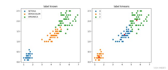
3. 效果展示

3.1. 有标签和无标签数据集

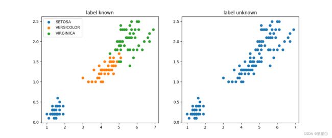
左图为有标签的数据集展示，右图是无标签的数据集展示，K-means算法是无监督的学习，没有类别标记，所以训练时不能指定标签，也就是右图所示的数据形式

3.2. 无标签与训练结果对比

左图为有标签的数据集，右图是经过k-means算法训练之后的结果演示，类别为3类，中心叉号代表每个类别的质心点

DBSCAN算法

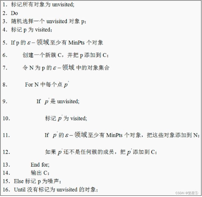
1. 理论基础

• 核心对象：若某个点的密度达到算法设定的阈值则其为核心点（即 r 邻域内点的数量不小于 minPts）

• ϵ-邻域的距离阈值：设定的半径r

• 直接密度可达：若某点p在点q的 r 邻域内，且q是核心点，则p-q直接密度可达

• 密度可达：若有一个点的序列q0、q1、…qk，对任意qi-qi-1是直接密度可达的 ，则称从q0到qk密度可达，这实际上是直接密度可达的传播

• 密度相连：若从某核心点p出发，点q和点k都是密度可达的 ，则称点q和点k是密度相连的。

• 边界点：属于某一个类的非核心点，不能发展下线了

• 直接密度可达：若某点p在点q的 r 邻域内，且q是核心点则p-q直接密度可达

• 工作流程：
  

• 优点：

  1. 不需要指定簇个数
  2. 可以发现任意形状的簇
  3. 擅长找到离群点（检测任务）
  4. 两个参数

• 缺点：

  1. 高维数据有些困难（可以做降维）
  2. 参数难以选择（参数对结果的影响非常大）
  3. Sklearn中效率很慢（数据削减策略）