NNDL 作业3：分别使用numpy和pytorch实现FNN例题

目录

题目

一、过程推导 - 了解BP原理

二、数值计算 - 手动计算，掌握细节

三、代码实现 - numpy手推 + pytorch自动

1、对比【numpy】和【pytorch】程序，总结并陈述。

2、激活函数Sigmoid用PyTorch自带函数torch.sigmoid()，观察、总结并陈述。

3、激活函数Sigmoid改变为Relu，观察、总结并陈述。

4、损失函数MSE用PyTorch自带函数 t.nn.MSELoss()替代，观察、总结并陈述。

5、损失函数MSE改变为交叉熵，观察、总结并陈述。

6、改变步长，训练次数，观察、总结并陈述。

7、权值w1-w8初始值换为随机数，对比“指定权值”的结果，观察、总结并陈述。

8、权值w1-w8初始值换为0，观察、总结并陈述。

四、全面总结反向传播原理和编码实现，认真写心得体会。

---

题目

一、过程推导 - 了解BP原理

西瓜书相关内容：

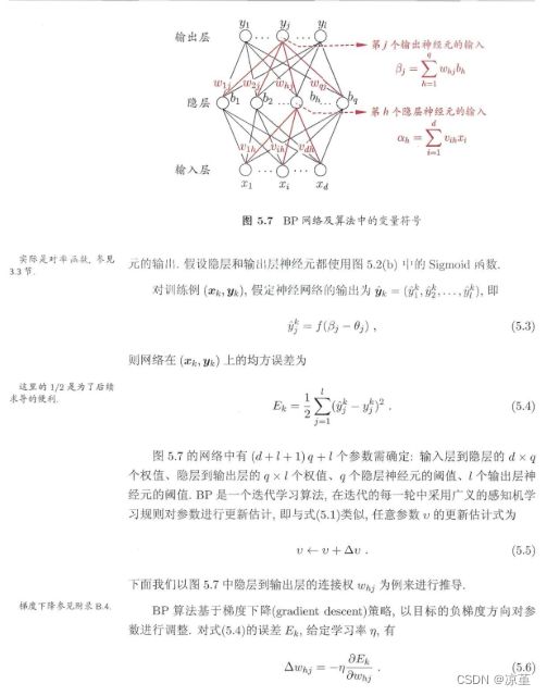
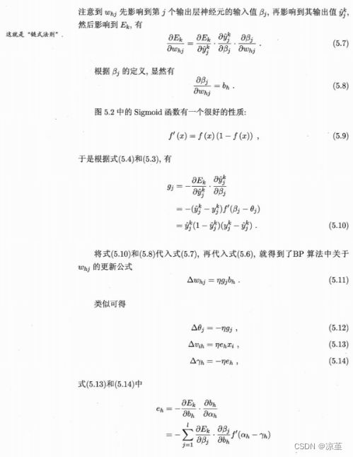
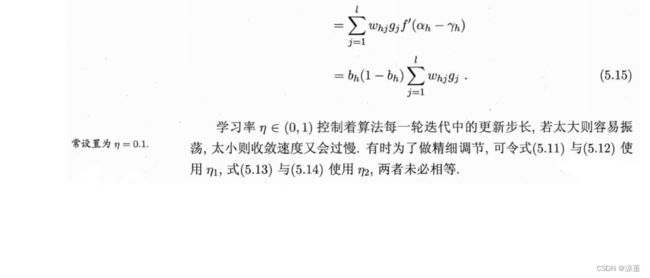
由此可得：

 

二、数值计算 - 手动计算，掌握细节

 

 
三、代码实现 - numpy手推 + pytorch自动

1、对比【numpy】和【pytorch】程序，总结并陈述。

使用numpy实现

import numpy as np
 
w1, w2, w3, w4, w5, w6, w7, w8 = 0.2, -0.4, 0.5, 0.6, 0.1, -0.5, -0.3, 0.8
x1, x2 = 0.5, 0.3
y1, y2 = 0.23, -0.07
print("输入值 x0, x1:")
print(x1, x2)
print("输出值 y0, y1:")
print(y1, y2)
 
 
def sigmoid(z):
    a = 1 / (1 + np.exp(-z))
    return a
 
 
def forward_propagate(x1, x2, y1, y2, w1, w2, w3, w4, w5, w6, w7, w8):
    in_h1 = w1 * x1 + w3 * x2
    out_h1 = sigmoid(in_h1)
    in_h2 = w2 * x1 + w4 * x2
    out_h2 = sigmoid(in_h2)
 
    in_o1 = w5 * out_h1 + w7 * out_h2
    out_o1 = sigmoid(in_o1)
    in_o2 = w6 * out_h1 + w8 * out_h2
    out_o2 = sigmoid(in_o2)
 
    print("正向计算:预测值o1 ,o2为")
    print(round(out_o1, 5), round(out_o2, 5))
 
    error = (1 / 2) * (out_o1 - y1) ** 2 + (1 / 2) * (out_o2 - y2) ** 2
 
    print("损失函数(均方误差)：",round(error, 5))
 
    return out_o1, out_o2, out_h1, out_h2
 
 
def back_propagate(out_o1, out_o2, out_h1, out_h2):
    # 反向传播
    d_o1 = out_o1 - y1
    d_o2 = out_o2 - y2
 
    d_w5 = d_o1 * out_o1 * (1 - out_o1) * out_h1
    d_w7 = d_o1 * out_o1 * (1 - out_o1) * out_h2
    d_w6 = d_o2 * out_o2 * (1 - out_o2) * out_h1
    d_w8 = d_o2 * out_o2 * (1 - out_o2) * out_h2
 
    d_w1 = (d_o1 * out_h1 * (1 - out_h1) * w5 + d_o2 * out_o2 * (1 - out_o2) * w6) * out_h1 * (1 - out_h1) * x1
    d_w3 = (d_o1 * out_h1 * (1 - out_h1) * w5 + d_o2 * out_o2 * (1 - out_o2) * w6) * out_h1 * (1 - out_h1) * x2
    d_w2 = (d_o1 * out_h1 * (1 - out_h1) * w7 + d_o2 * out_o2 * (1 - out_o2) * w8) * out_h2 * (1 - out_h2) * x1
    d_w4 = (d_o1 * out_h1 * (1 - out_h1) * w7 + d_o2 * out_o2 * (1 - out_o2) * w8) * out_h2 * (1 - out_h2) * x2
 
    print("反向传播：误差传给每个权值", round(d_w1, 5), round(d_w2, 5), round(d_w3, 5), round(d_w4, 5), round(d_w5, 5), round(d_w6, 5),
          round(d_w7, 5), round(d_w8, 5))
 
    return d_w1, d_w2, d_w3, d_w4, d_w5, d_w6, d_w7, d_w8
 
 
def update_w(w1, w2, w3, w4, w5, w6, w7, w8):
    # 步长
    step = 1
    w1 = w1 - step * d_w1
    w2 = w2 - step * d_w2
    w3 = w3 - step * d_w3
    w4 = w4 - step * d_w4
    w5 = w5 - step * d_w5
    w6 = w6 - step * d_w6
    w7 = w7 - step * d_w7
    w8 = w8 - step * d_w8
    return w1, w2, w3, w4, w5, w6, w7, w8
 
 
if __name__ == "__main__":
 
    print("更新前的权值:",round(w1, 2), round(w2, 2), round(w3, 2), round(w4, 2), round(w5, 2), round(w6, 2), round(w7, 2),
          round(w8, 2))
 
    for i in range(1):
        print("第" + str(i+1) + "轮:")
        out_o1, out_o2, out_h1, out_h2 = forward_propagate(x1, x2, y1, y2, w1, w2, w3, w4, w5, w6, w7, w8)
        d_w1, d_w2, d_w3, d_w4, d_w5, d_w6, d_w7, d_w8 = back_propagate(out_o1, out_o2, out_h1, out_h2)
        w1, w2, w3, w4, w5, w6, w7, w8 = update_w(w1, w2, w3, w4, w5, w6, w7, w8)
 
    print("更新后的权值w:", round(w1, 2), round(w2, 2), round(w3, 2), round(w4, 2), round(w5, 2), round(w6, 2), round(w7, 2),

运行结果

输入值 x0, x1:
0.5 0.3
输出值 y0, y1:
0.23 -0.07
更新前的权值: 0.2 -0.4 0.5 0.6 0.1 -0.5 -0.3 0.8
第1轮:
正向计算:预测值o1 ,o2为
0.47695 0.5287
损失函数(均方误差)： 0.20971
反向传播：误差传给每个权值 -0.00843 0.01264 -0.00506 0.00758 0.03463 0.08387 0.03049 0.07384
更新后的权值w: 0.21 -0.41 0.51 0.59 0.07 -0.58 -0.33 0.73

使用pytorch实现

import torch
 
x1, x2 = torch.Tensor([0.5]), torch.Tensor([0.3])
y1, y2 = torch.Tensor([0.23]), torch.Tensor([-0.07])
print("=====输入值：x1, x2；真实输出值：y1, y2=====")
print(x1, x2, y1, y2)
w1, w2, w3, w4, w5, w6, w7, w8 = torch.Tensor([0.2]), torch.Tensor([-0.4]), torch.Tensor([0.5]), torch.Tensor(
    [0.6]), torch.Tensor([0.1]), torch.Tensor([-0.5]), torch.Tensor([-0.3]), torch.Tensor([0.8])  # 权重初始值
w1.requires_grad = True
w2.requires_grad = True
w3.requires_grad = True
w4.requires_grad = True
w5.requires_grad = True
w6.requires_grad = True
w7.requires_grad = True
w8.requires_grad = True
 
 
def sigmoid(z):
    a = 1 / (1 + torch.exp(-z))
    return a
 
 
def forward_propagate(x1, x2):
    in_h1 = w1 * x1 + w3 * x2
    out_h1 = sigmoid(in_h1)  # out_h1 = torch.sigmoid(in_h1)
    in_h2 = w2 * x1 + w4 * x2
    out_h2 = sigmoid(in_h2)  # out_h2 = torch.sigmoid(in_h2)
 
    in_o1 = w5 * out_h1 + w7 * out_h2
    out_o1 = sigmoid(in_o1)  # out_o1 = torch.sigmoid(in_o1)
    in_o2 = w6 * out_h1 + w8 * out_h2
    out_o2 = sigmoid(in_o2)  # out_o2 = torch.sigmoid(in_o2)
 
    print("正向计算：o1 ,o2")
    print(out_o1.data, out_o2.data)
 
    return out_o1, out_o2
 
 
def loss_fuction(x1, x2, y1, y2):  # 损失函数
    y1_pred, y2_pred = forward_propagate(x1, x2)  # 前向传播
    loss = (1 / 2) * (y1_pred - y1) ** 2 + (1 / 2) * (y2_pred - y2) ** 2  # 考虑 ： t.nn.MSELoss()
    print("损失函数（均方误差）：", loss.item())
    return loss
 
 
def update_w(w1, w2, w3, w4, w5, w6, w7, w8):
    # 步长
    step = 1
    w1.data = w1.data - step * w1.grad.data
    w2.data = w2.data - step * w2.grad.data
    w3.data = w3.data - step * w3.grad.data
    w4.data = w4.data - step * w4.grad.data
    w5.data = w5.data - step * w5.grad.data
    w6.data = w6.data - step * w6.grad.data
    w7.data = w7.data - step * w7.grad.data
    w8.data = w8.data - step * w8.grad.data
    w1.grad.data.zero_()  # 注意：将w中所有梯度清零
    w2.grad.data.zero_()
    w3.grad.data.zero_()
    w4.grad.data.zero_()
    w5.grad.data.zero_()
    w6.grad.data.zero_()
    w7.grad.data.zero_()
    w8.grad.data.zero_()
    return w1, w2, w3, w4, w5, w6, w7, w8
 
 
if __name__ == "__main__":
 
    print("=====更新前的权值=====")
    print(w1.data, w2.data, w3.data, w4.data, w5.data, w6.data, w7.data, w8.data)
 
    for i in range(1):
        print("=====第" + str(i) + "轮=====")
        L = loss_fuction(x1, x2, y1, y2)  # 前向传播，求 Loss，构建计算图
        L.backward()  # 自动求梯度，不需要人工编程实现。反向传播，求出计算图中所有梯度存入w中
        print("\tgrad W: ", round(w1.grad.item(), 2), round(w2.grad.item(), 2), round(w3.grad.item(), 2),
              round(w4.grad.item(), 2), round(w5.grad.item(), 2), round(w6.grad.item(), 2), round(w7.grad.item(), 2),
              round(w8.grad.item(), 2))
        w1, w2, w3, w4, w5, w6, w7, w8 = update_w(w1, w2, w3, w4, w5, w6, w7, w8)
 
    print("更新后的权值")
    print(w1.data, w2.data, w3.data, w4.data, w5.data, w6.data, w7.data, w8.data)

运行结果

=====输入值：x1, x2；真实输出值：y1, y2=====
tensor([0.5000]) tensor([0.3000]) tensor([0.2300]) tensor([-0.0700])
=====更新前的权值=====
tensor([0.2000]) tensor([-0.4000]) tensor([0.5000]) tensor([0.6000]) tensor([0.1000]) tensor([-0.5000]) tensor([-0.3000]) tensor([0.8000])
=====第0轮=====
正向计算：o1 ,o2
tensor([0.4769]) tensor([0.5287])
损失函数（均方误差）： 0.2097097933292389
        grad W:  -0.01 0.01 -0.01 0.01 0.03 0.08 0.03 0.07
更新后的权值
tensor([0.2084]) tensor([-0.4126]) tensor([0.5051]) tensor([0.5924]) tensor([0.0654]) tensor([-0.5839]) tensor([-0.3305]) tensor([0.7262])

通过观察发现，两种方法的结果都十分相近，因此可认为两种方法的求解效果基本相同。但是numpy相对复杂，也不太系统，而pytorch实现通过调用函数代码较为简单。

2、激活函数Sigmoid用PyTorch自带函数torch.sigmoid()，观察、总结并陈述。

训练50轮：

正向计算：o1 ,o2
tensor([0.2758]) tensor([0.1304])
损失函数（均方误差）： 0.02112446539103985
        grad W:  -0.01 -0.0 -0.0 -0.0 0.01 0.01 0.0 0.01
更新后的权值
tensor([0.7606]) tensor([-0.3133]) tensor([0.8363]) tensor([0.6520]) tensor([-0.7251]) tensor([-2.3611]) tensor([-0.9798]) tensor([-0.7355])

训练100轮：

=====第99轮=====
正向计算：o1 ,o2
tensor([0.2378]) tensor([0.0736])
损失函数（均方误差）： 0.010342842899262905
        grad W:  -0.0 -0.0 -0.0 -0.0 0.0 0.01 0.0 0.01
更新后的权值
tensor([0.9865]) tensor([-0.2037]) tensor([0.9719]) tensor([0.7178]) tensor([-0.8628]) tensor([-2.8459]) tensor([-1.0866]) tensor([-1.1112])

Sigmoid函数的导数是其本身的函数，由上可知，使用Sigmoid函数和使用Pytorch自带函数torch.sigmoid()没较为明显的差距。

3、激活函数Sigmoid改变为Relu，观察、总结并陈述。

训练50轮：

=====第49轮=====
正向计算：o1 ,o2
tensor([0.2300]) tensor([0.])
损失函数（均方误差）： 0.0024500000290572643
        grad W:  -0.0 0.0 -0.0 0.0 -0.0 0.0 0.0 0.0
更新后的权值
tensor([0.4287]) tensor([-0.4000]) tensor([0.6372]) tensor([0.6000]) tensor([0.5672]) tensor([-0.5000]) tensor([-0.3000]) tensor([0.8000])

训练100轮：

=====第99轮=====
正向计算：o1 ,o2
tensor([0.2300]) tensor([0.])
损失函数（均方误差）： 0.0024500000290572643
        grad W:  -0.0 0.0 -0.0 0.0 -0.0 0.0 0.0 0.0
更新后的权值
tensor([0.4287]) tensor([-0.4000]) tensor([0.6372]) tensor([0.6000]) tensor([0.5672]) tensor([-0.5000]) tensor([-0.3000]) tensor([0.8000])

Relu函数其实就是分段的线性函数，作用是把所有的负值都变为0，而正值保持不变。

Relu激活函数收敛速度要优于使用sigmoid激活函数。

4、损失函数MSE用PyTorch自带函数 t.nn.MSELoss()替代，观察、总结并陈述。

def loss_fuction(x1, x2, y1, y2):  # 损失函数
    y1_pred, y2_pred = forward_propagate(x1, x2)  # 前向传播
    # loss = (1 / 2) * (y1_pred - y1) ** 2 + (1 / 2) * (y2_pred - y2) ** 2  # 考虑 ： t.nn.MSELoss()
    loss = torch.nn.MSELoss()
    loss1 = loss(y1_pred,y1)
    loss2 = loss(y2_pred,y2)
    loss = loss1 + loss2
    print("损失函数（均方误差）：", loss.item())
    return loss

训练50轮：

=====第49轮=====
正向计算：o1 ,o2
tensor([0.2300]) tensor([0.])
损失函数（均方误差）： 0.004900000058114529
        grad W:  -0.0 0.0 -0.0 0.0 -0.0 0.0 0.0 0.0
更新后的权值
tensor([0.4236]) tensor([-0.4000]) tensor([0.6342]) tensor([0.6000]) tensor([0.5720]) tensor([-0.5000]) tensor([-0.3000]) tensor([0.8000])

训练100轮：

=====第99轮=====
正向计算：o1 ,o2
tensor([0.2300]) tensor([0.])
损失函数（均方误差）： 0.004900000058114529
        grad W:  -0.0 0.0 -0.0 0.0 -0.0 0.0 0.0 0.0
更新后的权值
tensor([0.4236]) tensor([-0.4000]) tensor([0.6342]) tensor([0.6000]) tensor([0.5720]) tensor([-0.5000]) tensor([-0.3000]) tensor([0.8000])

MSELoss是均方误差，是预测值与真实值之差的平方和的平均值。

通过观察结果发现自带函数和编写的函数运行结果相同。

5、损失函数MSE改变为交叉熵，观察、总结并陈述。

def loss_fuction(x1, x2, y1, y2):
    y1_pred, y2_pred = forward_propagate(x1, x2)
    loss_func = torch.nn.CrossEntropyLoss() # 创建交叉熵损失函数
    y_pred = torch.stack([y1_pred, y2_pred], dim=1)
    y = torch.stack([y1, y2], dim=1)
    loss = loss_func(y_pred, y) # 计算
    print("损失函数（交叉熵损失）：", loss.item())
    return loss

训练50轮：

=====第49轮=====
正向计算：o1 ,o2
tensor([13.3109]) tensor([0.])
损失函数（交叉熵损失）： -0.9317622780799866
        grad W:  -0.17 0.0 -0.1 0.0 -0.2 0.0 0.0 0.0
更新后的权值
tensor([4.1027]) tensor([-0.4000]) tensor([2.8416]) tensor([0.6000]) tensor([4.9657]) tensor([-0.5000]) tensor([-0.3000]) tensor([0.8000])

训练100轮;

=====第99轮=====
正向计算：o1 ,o2
tensor([727.1639]) tensor([0.])
损失函数（交叉熵损失）： -50.9014778137207
        grad W:  -1.24 0.0 -0.74 0.0 -1.44 0.0 0.0 0.0
更新后的权值
tensor([31.3506]) tensor([-0.4000]) tensor([19.1903]) tensor([0.6000]) tensor([36.7545]) tensor([-0.5000]) tensor([-0.3000]) tensor([0.8000])

改为交叉熵之后损失函数出现负数。

6、改变步长，训练次数，观察、总结并陈述。

步长为0.5

训练50轮：

=====第49轮=====
正向计算：o1 ,o2
tensor([0.2758]) tensor([0.1304])
损失函数（均方误差）： 0.0422489307820797
        grad W:  -0.01 -0.01 -0.01 -0.0 0.01 0.03 0.01 0.02
更新后的权值
tensor([0.7606]) tensor([-0.3133]) tensor([0.8363]) tensor([0.6520]) tensor([-0.7251]) tensor([-2.3611]) tensor([-0.9798]) tensor([-0.7355])

训练100轮：

=====第99轮=====
正向计算：o1 ,o2
tensor([0.2378]) tensor([0.0736])
损失函数（均方误差）： 0.02068568579852581
        grad W:  -0.01 -0.0 -0.0 -0.0 0.0 0.01 0.0 0.01
更新后的权值
tensor([0.9865]) tensor([-0.2037]) tensor([0.9719]) tensor([0.7178]) tensor([-0.8628]) tensor([-2.8459]) tensor([-1.0866]) tensor([-1.1112])

步长为3

训练50轮：

=====第49轮=====
正向计算：o1 ,o2
tensor([0.2283]) tensor([0.0290])
损失函数（均方误差）： 0.009809560142457485
        grad W:  -0.0 -0.0 -0.0 -0.0 -0.0 0.0 -0.0 0.0
更新后的权值
tensor([1.2860]) tensor([-0.0748]) tensor([1.1516]) tensor([0.7951]) tensor([-0.8526]) tensor([-3.5755]) tensor([-1.0837]) tensor([-1.6757])

训练100轮：

=====第99轮=====
正向计算：o1 ,o2
tensor([0.2293]) tensor([0.0157])
损失函数（均方误差）： 0.007349265739321709
        grad W:  -0.0 -0.0 -0.0 -0.0 -0.0 0.0 -0.0 0.0
更新后的权值
tensor([1.4843]) tensor([0.0442]) tensor([1.2706]) tensor([0.8665]) tensor([-0.8113]) tensor([-3.9912]) tensor([-1.0526]) tensor([-1.9894])

如果选取合适的step并不会影响最优解的取得，反而会减少迭代的次数，提高时间效率。

7、权值w1-w8初始值换为随机数，对比“指定权值”的结果，观察、总结并陈述。

import torch
torch.manual_seed(20)

x1, x2 = torch.Tensor([0.5]), torch.Tensor([0.3])
y1, y2 = torch.Tensor([0.23]), torch.Tensor([-0.07])
print("=====输入值：x1, x2；真实输出值：y1, y2=====")
print(x1, x2, y1, y2)

w1, w2, w3, w4, w5, w6, w7, w8 =torch.rand(1), torch.rand(1), torch.rand(1), torch.rand(1), torch.rand(1),torch.rand(1), torch.rand(1), torch.rand(1)
w1.requires_grad = True
w2.requires_grad = True
w3.requires_grad = True
w4.requires_grad = True
w5.requires_grad = True
w6.requires_grad = True
w7.requires_grad = True
w8.requires_grad = True


def sigmoid(z):
    a = 1 / (1 + torch.exp(-z))
    return a


def forward_propagate(x1, x2):
    in_h1 = w1 * x1 + w3 * x2
    out_h1 = torch.relu(in_h1)  # out_h1 = torch.sigmoid(in_h1)
    in_h2 = w2 * x1 + w4 * x2
    out_h2 = torch.relu(in_h2)  # out_h2 = torch.sigmoid(in_h2)
    in_o1 = w5 * out_h1 + w7 * out_h2
    out_o1 = torch.relu(in_o1)  # out_o1 = torch.sigmoid(in_o1)
    in_o2 = w6 * out_h1 + w8 * out_h2
    out_o2 = torch.relu(in_o2)  # out_o2 = torch.sigmoid(in_o2)

    print("正向计算：o1 ,o2")
    print(out_o1.data, out_o2.data)

    return out_o1, out_o2


def loss_fuction(x1, x2, y1, y2):  # 损失函数
    y1_pred, y2_pred = forward_propagate(x1, x2)  # 前向传播
    loss = torch.nn.CrossEntropyLoss()  # 考虑 ： t.nn.MSELoss()
    y_pred = torch.stack([y1_pred, y2_pred], dim=1)
    y = torch.stack([y1, y2], dim=1)
    loss = loss(y_pred,y)
    print("损失函数（CrossEntropyLoss)：", loss.item())
    return loss


def update_w(w1, w2, w3, w4, w5, w6, w7, w8):
    # 步长
    step = 2
    w1.data = w1.data - step * w1.grad.data
    w2.data = w2.data - step * w2.grad.data
    w3.data = w3.data - step * w3.grad.data
    w4.data = w4.data - step * w4.grad.data
    w5.data = w5.data - step * w5.grad.data
    w6.data = w6.data - step * w6.grad.data
    w7.data = w7.data - step * w7.grad.data
    w8.data = w8.data - step * w8.grad.data
    w1.grad.data.zero_()  # 注意：将w中所有梯度清零
    w2.grad.data.zero_()
    w3.grad.data.zero_()
    w4.grad.data.zero_()
    w5.grad.data.zero_()
    w6.grad.data.zero_()
    w7.grad.data.zero_()
    w8.grad.data.zero_()
    return w1, w2, w3, w4, w5, w6, w7, w8


if __name__ == "__main__":

    print("=====更新前的权值=====")
    print(w1.data, w2.data, w3.data, w4.data, w5.data, w6.data, w7.data, w8.data)

    for i in range(2):
        print("=====第" + str(i) + "轮=====")
        L = loss_fuction(x1, x2, y1, y2)  # 前向传播，求 Loss，构建计算图
        L.backward()  # 自动求梯度，不需要人工编程实现。反向传播，求出计算图中所有梯度存入w中
        print("\tgrad W: ", round(w1.grad.item(), 2), round(w2.grad.item(), 2), round(w3.grad.item(), 2),
              round(w4.grad.item(), 2), round(w5.grad.item(), 2), round(w6.grad.item(), 2), round(w7.grad.item(), 2),
              round(w8.grad.item(), 2))
        w1, w2, w3, w4, w5, w6, w7, w8 = update_w(w1, w2, w3, w4, w5, w6, w7, w8)

    print("更新后的权值")
    print(w1.data, w2.data, w3.data, w4.data, w5.data, w6.data, w7.data, w8.data)

训练50轮：

=====第49轮=====
正向计算：o1 ,o2
tensor([1648.7810]) tensor([0.])
损失函数（CrossEntropyLoss)： -115.4146728515625
        grad W:  -1.1 -1.5 -0.66 -0.9 -1.29 0.0 -1.75 0.0
更新后的权值
tensor([29.0125]) tensor([39.6298]) tensor([17.8853]) tensor([24.0010]) tensor([34.0791]) tensor([0.2528]) tensor([46.3349]) tensor([-0.2410])

训练100轮：

=====第99轮=====
正向计算：o1 ,o2
tensor([4218611.]) tensor([0.])
损失函数（CrossEntropyLoss)： -295302.78125
        grad W:  -55.78 -75.84 -33.47 -45.5 -65.05 0.0 -88.44 0.0
更新后的权值
tensor([1477.9680]) tensor([2009.5591]) tensor([887.2587]) tensor([1205.9587]) tensor([1723.8379]) tensor([0.2528]) tensor([2343.6436]) tensor([-0.2410])

权重的初始化不会影响收敛的结果，均方误差的下降速度与指定权值时相比有所降低，收敛速度小于指定权值。

8、权值w1-w8初始值换为0，观察、总结并陈述。

将tensor中的数全部换为0

训练100轮：

=====第99轮=====
正向计算：o1 ,o2
tensor([0.]) tensor([0.])
损失函数（CrossEntropyLoss)： 0.1109035536646843
        grad W:  0.0 0.0 0.0 0.0 0.0 0.0 0.0 0.0
更新后的权值
tensor([0.]) tensor([0.]) tensor([0.]) tensor([0.]) tensor([0.]) tensor([0.]) tensor([0.]) tensor([0.])

权重初始值只影响收敛速度，并不会影响收敛结果。

四、全面总结反向传播原理和编码实现，认真写心得体会。

首先回顾了反向传播的计算流程，自己手推一遍真的让人印象深刻。

其次就是通过修改代码中激活函数、损失函数、步长、训练次数、权重等的值，运行观察了修改这些值对收敛速度、结果的影响。大部分的修改都是影响了收敛的速度，但它们的结果都大致相同。

参考文献：

NNDL 作业3：分别使用numpy和pytorch实现FNN例题_HBU_David的博客-CSDN博客

【2021-2022 春学期】人工智能-作业2：例题程序复现_HBU_David的博客-CSDN博客

【2021-2022 春学期】人工智能-作业3：例题程序复现 PyTorch版_HBU_David的博客-CSDN博客

【人工智能导论：模型与算法】MOOC 8.3 误差后向传播(BP) 例题 编程验证 Pytorch版本 - HBU_DAVID - 博客园

BP神经网络原理（详细推导）_Sun-sky的博客-CSDN博客_bp神经网络原理