python主成分分析_主成分分析(PCA)Python代码实现

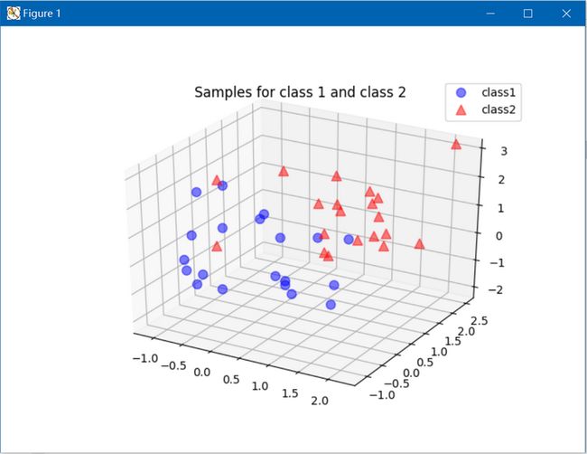
1. 随机生成3行*40列的数据集，每一列代表一个样本，前20列属于类1，后20列属于类2；每一个样本特征长度为3；

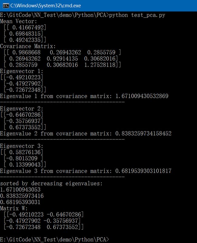
2. 计算每行均值；

3. 计算协方差矩阵，产生一个3行*3列的矩阵；

4. 由协方差矩阵计算特征向量和特征值；

5. 按降序排序特征值和特征向量；

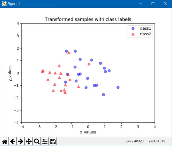
6. 选择第一主成分和第二主成分组成一个新的3行*2列的矩阵；

7. 根据产生的3行*2列矩阵重建原有数据集。

Python代码如下：

# reference: http://sebastianraschka.com/Articles/2014_pca_step_by_step.html

import numpy as np

from matplotlib import pyplot as plt

from mpl_toolkits.mplot3d import Axes3D

from mpl_toolkits.mplot3d import proj3d

from matplotlib.patches import FancyArrowPatch

# 1. generate 40 3-dimensional samples randomly drawn from a multivariate Gaussian distribution

np.random.seed(1) # random seed for consistency

mu_vec1 = np.array([0,0,0])

cov_mat1 = np.array([[1,0,0],[0,1,0],[0,0,1]])

class1_sample = np.random.multivariate_normal(mu_vec1, cov_mat1, 20).T

assert class1_sample.shape == (3,20), "The matrix has not the dimensions 3x20"

#print("class1_sample:\n", class1_sample)

mu_vec2 = np.array([1,1,1])

cov_mat2 = np.array([[1,0,0],[0,1,0],[0,0,1]])

class2_sample = np.random.multivariate_normal(mu_vec2, cov_mat2, 20).T

assert class2_sample.shape == (3,20), "The matrix has not the dimensions 3x20"

fig = plt.figure(figsize=(8,8))

ax = fig.add_subplot(111, projection='3d')

plt.rcParams['legend.fontsize'] = 10

ax.plot(class1_sample[0,:], class1_sample[1,:], class1_sample[2,:], 'o', markersize=8, color='blue', alpha=0.5, label='class1')

ax.plot(class2_sample[0,:], class2_sample[1,:], class2_sample[2,:], '^', markersize=8, alpha=0.5, color='red', label='class2')

plt.title('Samples for class 1 and class 2')

ax.legend(loc='upper right')

plt.show()

# Taking the whole dataset ignoring the class labels

all_samples = np.concatenate((class1_sample, class2_sample), axis=1)

assert all_samples.shape == (3,40), "The matrix has not the dimensions 3x40"

# 2. Computing the d-dimensional mean vector

mean_x = np.mean(all_samples[0,:])

mean_y = np.mean(all_samples[1,:])

mean_z = np.mean(all_samples[2,:])

mean_vector = np.array([[mean_x],[mean_y],[mean_z]])

print('Mean Vector:\n', mean_vector)

# 3. Computing the Covariance Matrix

cov_mat = np.cov([all_samples[0,:],all_samples[1,:],all_samples[2,:]])

print('Covariance Matrix:\n', cov_mat)

# 4. Computing eigenvectors and corresponding eigenvalues

eig_val_cov, eig_vec_cov = np.linalg.eig(cov_mat)

for i in range(len(eig_val_cov)):

eigvec_cov = eig_vec_cov[:,i].reshape(1,3).T

print('Eigenvector {}: \n{}'.format(i+1, eigvec_cov))

print('Eigenvalue {} from covariance matrix: {}'.format(i+1, eig_val_cov[i]))

print(40 * '-')

# Visualizing the eigenvectors

class Arrow3D(FancyArrowPatch):

def __init__(self, xs, ys, zs, *args, **kwargs):

FancyArrowPatch.__init__(self, (0,0), (0,0), *args, **kwargs)

self._verts3d = xs, ys, zs

def draw(self, renderer):

xs3d, ys3d, zs3d = self._verts3d

xs, ys, zs = proj3d.proj_transform(xs3d, ys3d, zs3d, renderer.M)

self.set_positions((xs[0],ys[0]),(xs[1],ys[1]))

FancyArrowPatch.draw(self, renderer)

fig = plt.figure(figsize=(7,7))

ax = fig.add_subplot(111, projection='3d')

ax.plot(all_samples[0,:], all_samples[1,:], all_samples[2,:], 'o', markersize=8, color='green', alpha=0.2)

ax.plot([mean_x], [mean_y], [mean_z], 'o', markersize=10, color='red', alpha=0.5)

for v in eig_vec_cov.T:

a = Arrow3D([mean_x, v[0]], [mean_y, v[1]], [mean_z, v[2]], mutation_scale=20, lw=3, arrowstyle="-|>", color="r")

ax.add_artist(a)

ax.set_xlabel('x_values')

ax.set_ylabel('y_values')

ax.set_zlabel('z_values')

plt.title('Eigenvectors')

plt.show()

# 5 Sorting the eigenvectors by decreasing eigenvalues

# Make a list of (eigenvalue, eigenvector) tuples

eig_pairs = [(np.abs(eig_val_cov[i]), eig_vec_cov[:,i]) for i in range(len(eig_val_cov))]

# Sort the (eigenvalue, eigenvector) tuples from high to low

eig_pairs.sort(key=lambda x: x[0], reverse=True)

print("eig_pairs:\n", eig_pairs)

# Visually confirm that the list is correctly sorted by decreasing eigenvalues

print("sorted by decreasing eigenvalues:")

for i in eig_pairs:

print(i[0])

# 6 Choosing k eigenvectors with the largest eigenvalues

matrix_w = np.hstack((eig_pairs[0][1].reshape(3,1), eig_pairs[1][1].reshape(3,1)))

print('Matrix W:\n', matrix_w)

# 7 Transforming the samples onto the new subspace

transformed = matrix_w.T.dot(all_samples)

assert transformed.shape == (2,40), "The matrix is not 2x40 dimensional."

plt.plot(transformed[0,0:20], transformed[1,0:20], 'o', markersize=7, color='blue', alpha=0.5, label='class1')

plt.plot(transformed[0,20:40], transformed[1,20:40], '^', markersize=7, color='red', alpha=0.5, label='class2')

plt.xlim([-4,4])

plt.ylim([-4,4])

plt.xlabel('x_values')

plt.ylabel('y_values')

plt.legend()

plt.title('Transformed samples with class labels')

plt.show()

执行结果如下：

GitHub：

https://github.com/fengbingchun/NN_Test