从零用JS来做人工智能

更新时间：2020年3月10日

1 环境准备

nodeJs
vscode或其他代码编辑器
Chrome浏览器或其他现代浏览器

tensorflow js 依赖，纯JS包，速度最慢

npm i @tensorflow/tfjs

【可选】构建C++底层包 版本控制4.0.0

npm i node-gyp [email protected]

【可选】tensorflow c++底层包，依赖C++底层包，速度比较快

npm i @tensorflow/tfjs-node

【可选】tensorflow gpu包，依赖C++底层包，速度最快，需要相关配置

npm i @tensorflow/tfjs-node-gpu

【可选】web应用打包工具 Parcel

npm install -g parcel-bundler

用法示例：parcel 路径/*.html

C:\Users\Administrator\Desktop\learnJS>parcel linear-regression/*
Server running at http://localhost:1234 
√  Built in 1.24s.

其他：中学数学知识，基础前端、神经网络等预备知识

2 基础篇

读文档永远是个好习惯
tensorflow API for JS
Google机械学习速成教程

2.1 点乘

import * as tf from '@tensorflow/tfjs';

//传统for循环
const input = [1, 2, 3, 4];
const w = [[1, 2, 3, 4], [2, 3, 4, 5], [3, 4, 5, 6], [4, 5, 6, 7]];
const output = [0, 0, 0, 0];

for(let i = 0; i< w.length; i++){
  for(let j = 0;j< input.length; j++){
    output[i] += input[j] * w[i][j];
  }
}

console.log(output);
//使用tensorflow实现点乘
tf.tensor(w).dot(tf.tensor(input)).print();

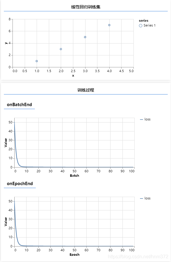
2.2 构建神经网络

• 准备线性回归训练数据
• 使用tfvis可视化训练数据

npm i @tensorflow/tfjs-vis -S

import * as tfvis from '@tensorflow/tfjs-vis'
window.onload = () => {
  const xs = [1, 2, 3, 4];
  const ys = [1, 3, 5, 7];

  tfvis.render.scatterplot(
    { name: '线性回归训练集' },
    { values: xs.map((x, i) => ({ x, y: ys[i] })) },
    //设置x,y轴范围
    { xAxisDomain: [0, 5], yAxisDomain: [0, 8] }
  );
};

• 初始化一个神经网络模型
• 为神经网络模型添加层
• 设计层的神经元个数和inputShape（单层单个神经元组成的神经网络）

import * as tf from '@tensorflow/tfjs';
//初始化连续模型
const model = tf.sequential();
model.add(tf.layers.dense( {units: 1, inputShape: [1]}))

• Google机器学期速成教程理解损失函数与均方误差
• 在tensorflow.js中设置损失函数：均方误差（MSE）

model.compile({ loss: tf.losses.meanSquaredError });

• Google机器学期速成教程理解优化器和随机梯度下降
• 在tensorflow.js中设置优化器：随机梯度下降（SGD）

model.compile({ loss: tf.losses.meanSquaredError, optimizer: tf.train.sgd(0.1)});

2.3 训练模型并可视化训练+预测

• 将训练数据转为tensor
• 训练模型
• 使用tfvis可视化

//package.json 加上下面的语句
"browserslist": ["last 1 Chrome version"]

import * as tf from '@tensorflow/tfjs';
import * as tfvis from '@tensorflow/tfjs-vis'

window.onload = async () => {
  const xs = [1, 2, 3, 4];
  const ys = [1, 3, 5, 7];

  tfvis.render.scatterplot(
    { name: '线性回归训练集' },
    { values: xs.map((x, i) => ({ x, y: ys[i] })) },
    //设置x,y轴范围
    { xAxisDomain: [0, 5], yAxisDomain: [0, 8] }
  );

  //初始化连续模型
  const model = tf.sequential();
  model.add(tf.layers.dense({ units: 1, inputShape: [1] }))
  model.compile({ loss: tf.losses.meanSquaredError, optimizer: tf.train.sgd(0.01)});//sgd 学习率
  //转化为tensor变量
  const inputs = tf.tensor(xs);
  const labels = tf.tensor(ys);
  await model.fit(inputs, labels, {
    //小批量大小
    batchSize: 4,
    //迭代次数
    epochs: 100,
    //可视化
    callbacks: tfvis.show.fitCallbacks(
      {name:'训练过程'},
      ['loss']
      )
  });
};

• 将预测数据转为tensor
• 使用训练好的模型进行预测
• 将输出的tensor转为普通数据并显示

  //预测x为5的时候的y值
  const output = model.predict(tf.tensor([5]));
  alert('如果x为5，那么预测y为'  + output.dataSync()[0]);

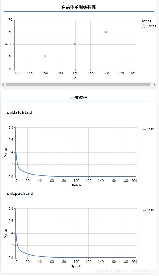
2.4 归一化

什么是归一化？

• 把大数量级特折转化到较小的数据集下，通常是[0,1]或[-1,1]
• 例子：身高体重预测、房价预测

为何要归一化？

• 绝大多数tensorflow.js模型都不是给特别大的数设计的
• 将不同数量级的特征转换到同一数量级，防止某个特征影响过大

操作步骤

• 准备身高特种训练数据并归一化
• 定义一个神经网络模型，训练模型并预测
• 将结果反归一化为正常数据

代码

import * as tf from '@tensorflow/tfjs';
import * as tfvis from '@tensorflow/tfjs-vis';

window.onload = async () => {
  const heights = [150, 160, 170];
  const weights = [40, 50, 60];

  //可视化
  tfvis.render.scatterplot(
    { name: '身高体重训练数据' },
    { values: heights.map((x, i) => ({ x, y: weights[i] })) },
    {
      xAxisDomain: [140, 180],
      yAxisDomain: [30, 70]
    }
  );

  //此处用到的归一化算法 减去最小值，再除以差值
  const inputs = tf.tensor(heights).sub(150).div(20);
  const labels = tf.tensor(weights).sub(40).div(10);

  //初始化连续模型
  const model = tf.sequential();
  model.add(tf.layers.dense({ units: 1, inputShape: [1] }))
  model.compile({ loss: tf.losses.meanSquaredError, optimizer: tf.train.sgd(0.1) });//sgd 学习率

  await model.fit(inputs, labels, {
    //小批量大小
    batchSize: 3,
    //迭代次数
    epochs: 200,
    //可视化
    callbacks: tfvis.show.fitCallbacks(
      { name: '训练过程' },
      ['loss']
    )
  });

  //预测身高为180的时候的体重
  const output = model.predict(tf.tensor([180]).sub(150).div(20));
  //反归一化
  alert('如果身高为180cm，那么预测体重为' + output.mul(10).add(40).dataSync()[0]) + 'kg';
};

训练过程

预测结果

2.5 逻辑回归

操作步骤

• 使用预先准备好的脚本生成二分类数据集，并进行可视化
• 定义模型结构：带有激活函数的单个神经元
• 训练模型并预测

生成数据集脚本代码
data.js

export function getData(numSamples) {
    let points = [];
  
    function genGauss(cx, cy, label) {
      for (let i = 0; i < numSamples / 2; i++) {
        let x = normalRandom(cx);
        let y = normalRandom(cy);
        points.push({ x, y, label });
      }
    }
  	//生成以(2,2)为中心label为1的 正态分布点
    genGauss(2, 2, 1);
    //生成以(-2,-2)为中心label为0的 正态分布点
    genGauss(-2, -2, 0);
    return points;
  }
  
  /**
   * Samples from a normal distribution. Uses the seedrandom library as the
   * random generator.
   *
   * @param mean The mean. Default is 0.
   * @param variance The variance. Default is 1.
   */
  function normalRandom(mean = 0, variance = 1) {
    let v1, v2, s;
    do {
      v1 = 2 * Math.random() - 1;
      v2 = 2 * Math.random() - 1;
      s = v1 * v1 + v2 * v2;
    } while (s > 1);
  
    let result = Math.sqrt(-2 * Math.log(s) / s) * v1;
    return mean + Math.sqrt(variance) * result;
  }

主函数
script.js

import * as tf from '@tensorflow/tfjs';
import * as tfvis from '@tensorflow/tfjs-vis';
import { getData } from './data.js';

window.onload = async () => {
  const data = getData(400);
  console.log(data);

  tfvis.render.scatterplot(
    { name: '逻辑回归训练数据' },
    {
      values: [
        data.filter(p => p.label === 1),
        data.filter(p => p.label === 0),
      ]
    }
  );

  const model = tf.sequential();
  model.add(tf.layers.dense({
    units: 1,
    inputShape: [2],
    activation: 'sigmoid'
  }));
  model.compile({
    loss: tf.losses.logLoss,
    optimizer: tf.train.adam(0.1)
  });

  const inputs = tf.tensor(data.map(p => [p.x, p.y]));
  const labels = tf.tensor(data.map(p => p.label));

  await model.fit(inputs, labels, {
    batchSize: 40,
    epochs: 20,
    callbacks: tfvis.show.fitCallbacks(
      { name: '训练效果' },
      ['loss']
    )
  });

  window.predict = (form) => {
    const pred = model.predict(tf.tensor([[form.x.value * 1, form.y.value * 1]]));
    alert(`预测结果：${pred.dataSync()[0]}`);
  };
};

前端代码
index.html

<script src="script.js">script>
<form action="" onsubmit="predict(this);return false;">
    x: <input type="text" name="x">
    y: <input type="text" name="y">
    <button type="submit">预测button>
form>

预测过程

进行预测

2.6 多层神经网络

2.6.1 XOR逻辑回归

神经网络在线演示网站
操作步骤

• 加载XOR数据集
• 定义模型结构：多层神经网络
• 训练模型并预测
  data.js

export function getData(numSamples) {
    let points = [];
  
    function genGauss(cx, cy, label) {
      for (let i = 0; i < numSamples / 2; i++) {
        let x = normalRandom(cx);
        let y = normalRandom(cy);
        points.push({ x, y, label });
      }
    }
  
    genGauss(2, 2, 0);
    genGauss(-2, -2, 0);
    genGauss(-2, 2, 1);
    genGauss(2, -2, 1);
    return points;
  }
  
  /**
   * Samples from a normal distribution. Uses the seedrandom library as the
   * random generator.
   *
   * @param mean The mean. Default is 0.
   * @param variance The variance. Default is 1.
   */
  function normalRandom(mean = 0, variance = 1) {
    let v1, v2, s;
    do {
      v1 = 2 * Math.random() - 1;
      v2 = 2 * Math.random() - 1;
      s = v1 * v1 + v2 * v2;
    } while (s > 1);
  
    let result = Math.sqrt(-2 * Math.log(s) / s) * v1;
    return mean + Math.sqrt(variance) * result;
  }

script.js

import * as tf from '@tensorflow/tfjs';
import * as tfvis from '@tensorflow/tfjs-vis';
import { getData } from './data.js';

window.onload = async () => {
    const data = getData(400);

    tfvis.render.scatterplot(
        { name: 'XOR 训练数据' },
        {
            values: [
                data.filter(p => p.label === 1),
                data.filter(p => p.label === 0),
            ]
        }
    );

    const model = tf.sequential();
    model.add(tf.layers.dense({
        units: 4,
        inputShape: [2],
        activation: 'relu'
    }));
    model.add(tf.layers.dense({
        units: 1,
        activation: 'sigmoid'
    }));
    model.compile({
        loss: tf.losses.logLoss,
        optimizer: tf.train.adam(0.1)
    });

    const inputs = tf.tensor(data.map(p => [p.x, p.y]));
    const labels = tf.tensor(data.map(p => p.label));

    await model.fit(inputs, labels, {
        epochs: 10,
        callbacks: tfvis.show.fitCallbacks(
            { name: '训练效果' },
            ['loss']
        )
    });

    window.predict = (form) => {
        const pred = model.predict(tf.tensor([[form.x.value * 1, form.y.value * 1]]));
        alert(`预测结果：${pred.dataSync()[0]}`);
    };
};

index.html

<script src="script.js">script>
<form action="" onsubmit="predict(this);return false;">
    x: <input type="text" name="x">
    y: <input type="text" name="y">
    <button type="submit">预测button>
form>

进行预测

2.7 多分类任务

操作步骤

• 加载IRIS数据集（训练集与验证集）
• 定义模型结构：带有softmax的多层神经网络
• 训练模型并预测
  代码
  数据集脚本 data.js

import * as tf from '@tensorflow/tfjs';

export const IRIS_CLASSES =
    ['山鸢尾', '变色鸢尾', '维吉尼亚鸢尾'];
export const IRIS_NUM_CLASSES = IRIS_CLASSES.length;

// Iris flowers data. Source:
//   https://archive.ics.uci.edu/ml/machine-learning-databases/iris/iris.data
const IRIS_DATA = [
  [5.1, 3.5, 1.4, 0.2, 0], [4.9, 3.0, 1.4, 0.2, 0], [4.7, 3.2, 1.3, 0.2, 0],
  [4.6, 3.1, 1.5, 0.2, 0], [5.0, 3.6, 1.4, 0.2, 0], [5.4, 3.9, 1.7, 0.4, 0],
  [4.6, 3.4, 1.4, 0.3, 0], [5.0, 3.4, 1.5, 0.2, 0], [4.4, 2.9, 1.4, 0.2, 0],
  [4.9, 3.1, 1.5, 0.1, 0], [5.4, 3.7, 1.5, 0.2, 0], [4.8, 3.4, 1.6, 0.2, 0],
  [4.8, 3.0, 1.4, 0.1, 0], [4.3, 3.0, 1.1, 0.1, 0], [5.8, 4.0, 1.2, 0.2, 0],
  [5.7, 4.4, 1.5, 0.4, 0], [5.4, 3.9, 1.3, 0.4, 0], [5.1, 3.5, 1.4, 0.3, 0],
  [5.7, 3.8, 1.7, 0.3, 0], [5.1, 3.8, 1.5, 0.3, 0], [5.4, 3.4, 1.7, 0.2, 0],
  [5.1, 3.7, 1.5, 0.4, 0], [4.6, 3.6, 1.0, 0.2, 0], [5.1, 3.3, 1.7, 0.5, 0],
  [4.8, 3.4, 1.9, 0.2, 0], [5.0, 3.0, 1.6, 0.2, 0], [5.0, 3.4, 1.6, 0.4, 0],
  [5.2, 3.5, 1.5, 0.2, 0], [5.2, 3.4, 1.4, 0.2, 0], [4.7, 3.2, 1.6, 0.2, 0],
  [4.8, 3.1, 1.6, 0.2, 0], [5.4, 3.4, 1.5, 0.4, 0], [5.2, 4.1, 1.5, 0.1, 0],
  [5.5, 4.2, 1.4, 0.2, 0], [4.9, 3.1, 1.5, 0.1, 0], [5.0, 3.2, 1.2, 0.2, 0],
  [5.5, 3.5, 1.3, 0.2, 0], [4.9, 3.1, 1.5, 0.1, 0], [4.4, 3.0, 1.3, 0.2, 0],
  [5.1, 3.4, 1.5, 0.2, 0], [5.0, 3.5, 1.3, 0.3, 0], [4.5, 2.3, 1.3, 0.3, 0],
  [4.4, 3.2, 1.3, 0.2, 0], [5.0, 3.5, 1.6, 0.6, 0], [5.1, 3.8, 1.9, 0.4, 0],
  [4.8, 3.0, 1.4, 0.3, 0], [5.1, 3.8, 1.6, 0.2, 0], [4.6, 3.2, 1.4, 0.2, 0],
  [5.3, 3.7, 1.5, 0.2, 0], [5.0, 3.3, 1.4, 0.2, 0], [7.0, 3.2, 4.7, 1.4, 1],
  [6.4, 3.2, 4.5, 1.5, 1], [6.9, 3.1, 4.9, 1.5, 1], [5.5, 2.3, 4.0, 1.3, 1],
  [6.5, 2.8, 4.6, 1.5, 1], [5.7, 2.8, 4.5, 1.3, 1], [6.3, 3.3, 4.7, 1.6, 1],
  [4.9, 2.4, 3.3, 1.0, 1], [6.6, 2.9, 4.6, 1.3, 1], [5.2, 2.7, 3.9, 1.4, 1],
  [5.0, 2.0, 3.5, 1.0, 1], [5.9, 3.0, 4.2, 1.5, 1], [6.0, 2.2, 4.0, 1.0, 1],
  [6.1, 2.9, 4.7, 1.4, 1], [5.6, 2.9, 3.6, 1.3, 1], [6.7, 3.1, 4.4, 1.4, 1],
  [5.6, 3.0, 4.5, 1.5, 1], [5.8, 2.7, 4.1, 1.0, 1], [6.2, 2.2, 4.5, 1.5, 1],
  [5.6, 2.5, 3.9, 1.1, 1], [5.9, 3.2, 4.8, 1.8, 1], [6.1, 2.8, 4.0, 1.3, 1],
  [6.3, 2.5, 4.9, 1.5, 1], [6.1, 2.8, 4.7, 1.2, 1], [6.4, 2.9, 4.3, 1.3, 1],
  [6.6, 3.0, 4.4, 1.4, 1], [6.8, 2.8, 4.8, 1.4, 1], [6.7, 3.0, 5.0, 1.7, 1],
  [6.0, 2.9, 4.5, 1.5, 1], [5.7, 2.6, 3.5, 1.0, 1], [5.5, 2.4, 3.8, 1.1, 1],
  [5.5, 2.4, 3.7, 1.0, 1], [5.8, 2.7, 3.9, 1.2, 1], [6.0, 2.7, 5.1, 1.6, 1],
  [5.4, 3.0, 4.5, 1.5, 1], [6.0, 3.4, 4.5, 1.6, 1], [6.7, 3.1, 4.7, 1.5, 1],
  [6.3, 2.3, 4.4, 1.3, 1], [5.6, 3.0, 4.1, 1.3, 1], [5.5, 2.5, 4.0, 1.3, 1],
  [5.5, 2.6, 4.4, 1.2, 1], [6.1, 3.0, 4.6, 1.4, 1], [5.8, 2.6, 4.0, 1.2, 1],
  [5.0, 2.3, 3.3, 1.0, 1], [5.6, 2.7, 4.2, 1.3, 1], [5.7, 3.0, 4.2, 1.2, 1],
  [5.7, 2.9, 4.2, 1.3, 1], [6.2, 2.9, 4.3, 1.3, 1], [5.1, 2.5, 3.0, 1.1, 1],
  [5.7, 2.8, 4.1, 1.3, 1], [6.3, 3.3, 6.0, 2.5, 2], [5.8, 2.7, 5.1, 1.9, 2],
  [7.1, 3.0, 5.9, 2.1, 2], [6.3, 2.9, 5.6, 1.8, 2], [6.5, 3.0, 5.8, 2.2, 2],
  [7.6, 3.0, 6.6, 2.1, 2], [4.9, 2.5, 4.5, 1.7, 2], [7.3, 2.9, 6.3, 1.8, 2],
  [6.7, 2.5, 5.8, 1.8, 2], [7.2, 3.6, 6.1, 2.5, 2], [6.5, 3.2, 5.1, 2.0, 2],
  [6.4, 2.7, 5.3, 1.9, 2], [6.8, 3.0, 5.5, 2.1, 2], [5.7, 2.5, 5.0, 2.0, 2],
  [5.8, 2.8, 5.1, 2.4, 2], [6.4, 3.2, 5.3, 2.3, 2], [6.5, 3.0, 5.5, 1.8, 2],
  [7.7, 3.8, 6.7, 2.2, 2], [7.7, 2.6, 6.9, 2.3, 2], [6.0, 2.2, 5.0, 1.5, 2],
  [6.9, 3.2, 5.7, 2.3, 2], [5.6, 2.8, 4.9, 2.0, 2], [7.7, 2.8, 6.7, 2.0, 2],
  [6.3, 2.7, 4.9, 1.8, 2], [6.7, 3.3, 5.7, 2.1, 2], [7.2, 3.2, 6.0, 1.8, 2],
  [6.2, 2.8, 4.8, 1.8, 2], [6.1, 3.0, 4.9, 1.8, 2], [6.4, 2.8, 5.6, 2.1, 2],
  [7.2, 3.0, 5.8, 1.6, 2], [7.4, 2.8, 6.1, 1.9, 2], [7.9, 3.8, 6.4, 2.0, 2],
  [6.4, 2.8, 5.6, 2.2, 2], [6.3, 2.8, 5.1, 1.5, 2], [6.1, 2.6, 5.6, 1.4, 2],
  [7.7, 3.0, 6.1, 2.3, 2], [6.3, 3.4, 5.6, 2.4, 2], [6.4, 3.1, 5.5, 1.8, 2],
  [6.0, 3.0, 4.8, 1.8, 2], [6.9, 3.1, 5.4, 2.1, 2], [6.7, 3.1, 5.6, 2.4, 2],
  [6.9, 3.1, 5.1, 2.3, 2], [5.8, 2.7, 5.1, 1.9, 2], [6.8, 3.2, 5.9, 2.3, 2],
  [6.7, 3.3, 5.7, 2.5, 2], [6.7, 3.0, 5.2, 2.3, 2], [6.3, 2.5, 5.0, 1.9, 2],
  [6.5, 3.0, 5.2, 2.0, 2], [6.2, 3.4, 5.4, 2.3, 2], [5.9, 3.0, 5.1, 1.8, 2],
];

/**
 * Convert Iris data arrays to `tf.Tensor`s.
 *
 * @param data The Iris input feature data, an `Array` of `Array`s, each element
 *   of which is assumed to be a length-4 `Array` (for petal length, petal
 *   width, sepal length, sepal width).
 * @param targets An `Array` of numbers, with values from the set {0, 1, 2}:
 *   representing the true category of the Iris flower. Assumed to have the same
 *   array length as `data`.
 * @param testSplit Fraction of the data at the end to split as test data: a
 *   number between 0 and 1.
 * @return A length-4 `Array`, with
 *   - training data as `tf.Tensor` of shape [numTrainExapmles, 4].
 *   - training one-hot labels as a `tf.Tensor` of shape [numTrainExamples, 3]
 *   - test data as `tf.Tensor` of shape [numTestExamples, 4].
 *   - test one-hot labels as a `tf.Tensor` of shape [numTestExamples, 3]
 */
function convertToTensors(data, targets, testSplit) {
  const numExamples = data.length;
  if (numExamples !== targets.length) {
    throw new Error('data and split have different numbers of examples');
  }

  // Randomly shuffle `data` and `targets`.
  const indices = [];
  for (let i = 0; i < numExamples; ++i) {
    indices.push(i);
  }
  tf.util.shuffle(indices);

  const shuffledData = [];
  const shuffledTargets = [];
  for (let i = 0; i < numExamples; ++i) {
    shuffledData.push(data[indices[i]]);
    shuffledTargets.push(targets[indices[i]]);
  }

  // Split the data into a training set and a tet set, based on `testSplit`.
  const numTestExamples = Math.round(numExamples * testSplit);
  const numTrainExamples = numExamples - numTestExamples;

  const xDims = shuffledData[0].length;

  // Create a 2D `tf.Tensor` to hold the feature data.
  const xs = tf.tensor2d(shuffledData, [numExamples, xDims]);

  // Create a 1D `tf.Tensor` to hold the labels, and convert the number label
  // from the set {0, 1, 2} into one-hot encoding (.e.g., 0 --> [1, 0, 0]).
  const ys = tf.oneHot(tf.tensor1d(shuffledTargets).toInt(), IRIS_NUM_CLASSES);

  // Split the data into training and test sets, using `slice`.
  const xTrain = xs.slice([0, 0], [numTrainExamples, xDims]);
  const xTest = xs.slice([numTrainExamples, 0], [numTestExamples, xDims]);
  const yTrain = ys.slice([0, 0], [numTrainExamples, IRIS_NUM_CLASSES]);
  const yTest = ys.slice([0, 0], [numTestExamples, IRIS_NUM_CLASSES]);
  return [xTrain, yTrain, xTest, yTest];
}

/**
 * Obtains Iris data, split into training and test sets.
 *
 * @param testSplit Fraction of the data at the end to split as test data: a
 *   number between 0 and 1.
 *
 * @param return A length-4 `Array`, with
 *   - training data as an `Array` of length-4 `Array` of numbers.
 *   - training labels as an `Array` of numbers, with the same length as the
 *     return training data above. Each element of the `Array` is from the set
 *     {0, 1, 2}.
 *   - test data as an `Array` of length-4 `Array` of numbers.
 *   - test labels as an `Array` of numbers, with the same length as the
 *     return test data above. Each element of the `Array` is from the set
 *     {0, 1, 2}.
 */
export function getIrisData(testSplit) {
  return tf.tidy(() => {
    const dataByClass = [];
    const targetsByClass = [];
    for (let i = 0; i < IRIS_CLASSES.length; ++i) {
      dataByClass.push([]);
      targetsByClass.push([]);
    }
    for (const example of IRIS_DATA) {
      const target = example[example.length - 1];
      const data = example.slice(0, example.length - 1);
      dataByClass[target].push(data);
      targetsByClass[target].push(target);
    }

    const xTrains = [];
    const yTrains = [];
    const xTests = [];
    const yTests = [];
    for (let i = 0; i < IRIS_CLASSES.length; ++i) {
      const [xTrain, yTrain, xTest, yTest] =
          convertToTensors(dataByClass[i], targetsByClass[i], testSplit);
      xTrains.push(xTrain);
      yTrains.push(yTrain);
      xTests.push(xTest);
      yTests.push(yTest);
    }

    const concatAxis = 0;
    return [
      tf.concat(xTrains, concatAxis), tf.concat(yTrains, concatAxis),
      tf.concat(xTests, concatAxis), tf.concat(yTests, concatAxis)
    ];
  });
}

scripts.js

import * as tf from '@tensorflow/tfjs';
import * as tfvis from '@tensorflow/tfjs-vis';
import { getIrisData, IRIS_CLASSES } from './data';

window.onload = async () => {
    //训练集特征 标签 验证集特征 标签
    const [xTrain, yTrain, xTest, yTest] = getIrisData(0.15);

    const model = tf.sequential();
    model.add(tf.layers.dense({
        units: 10,
        inputShape: [xTrain.shape[1]],
        activation: 'sigmoid'
    }));
    model.add(tf.layers.dense({
        units: 3,
        activation: 'softmax'
    }));

    model.compile({
        loss: 'categoricalCrossentropy',
        optimizer: tf.train.adam(0.1),
        metrics: ['accuracy']
    });

    await model.fit(xTrain, yTrain, {
        epochs: 100,
        validationData: [xTest, yTest],   //验证器
        callbacks: tfvis.show.fitCallbacks(
            { name: '训练效果' },
            ['loss', 'val_loss', 'acc', 'val_acc'],
            { callbacks: ['onEpochEnd'] }
        )
    });

    window.predict = (form) => {
        const input = tf.tensor([[
            form.a.value * 1,
            form.b.value * 1,
            form.c.value * 1,
            form.d.value * 1,
        ]]);
        const pred = model.predict(input);
        alert(`预测结果：${IRIS_CLASSES[pred.argMax(1).dataSync(0)]}`);
    };
};

前端页面 index.html

<script src="script.js">script>
<form action="" onsubmit="predict(this); return false;">
    花萼长度：<input type="text" name="a"><br>
    花萼宽度：<input type="text" name="b"><br>
    花瓣长度：<input type="text" name="c"><br>
    花瓣宽度：<input type="text" name="d"><br>
    <button type="submit">预测button>
form>

训练过程

进行预测

2.8 欠拟合与过拟合

什么是欠拟合？
简单来说就是数据集很复杂，模型太简单，导致数据无法拟合

什么是过拟合？

过拟合特征曲线

操作步骤

• 加载代有噪音的二分类数据集
• 使用不同神经网络演示欠拟合和过拟合
• 过拟合应对法：早停法、权重衰减、丢弃法