12 _Custom Models and Training with TensorFlow_3_MomentumOptimizers_ Batch Normalization

12 _Custom Models and Training with TensorFlow_tensor_ structure_Activation_Layers_huber_Loss_Metric
https://blog.csdn.net/Linli522362242/article/details/107294292

12 _Custom Models and Training with TensorFlow_2_progress_status_bar_Training Loops_concretehttps://blog.csdn.net/Linli522362242/article/details/107459161

Using TF Functions with tf.keras (or Not)

     By default, any custom function, layer, or model you use with tf.keras will automatically be converted to a TF Function; you do not need to do anything at all!

from sklearn.datasets import fetch_california_housing
from sklearn.model_selection import train_test_split
from sklearn.preprocessing import StandardScaler

housing = fetch_california_housing()
X_train_full, X_test, y_train_full, y_test = train_test_split(
    housing.data, housing.target.reshape(-1, 1), random_state=42
)
X_train, X_valid, y_train, y_valid = train_test_split(
    X_train_full, y_train_full, random_state=42,#If train_size is also None,it will be set to 0.25
)

scaler = StandardScaler()
X_train_scaled = scaler.fit_transform(X_train)
X_valid_scaled = scaler.transform(X_valid)
X_test_scaled = scaler.transform(X_test)


import tensorflow as tf
from tensorflow import keras
import numpy as np

# Custom Loss function ################################
def my_mse(y_true, y_pred):
    print("Tracing loss my_mse()")
    return tf.reduce_mean( tf.square(y_pred - y_true) )

# Custom metric function ##############################
def my_mae(y_true, y_pred):
    print("Tracing metric my_mae()")
    return tf.reduce_mean( tf.abs(y_pred - y_true) )

# Custom layer ########################################
class MyDense(keras.layers.Layer):
    def __init__(self, units, activation=None, **kwargs):
        super().__init__(**kwargs)
        self.units = units
        self.activation = keras.activations.get(activation)
        
    def build(self, input_shape):
        self.kernel = self.add_weight(name='kernel',
                                      shape=(input_shape[1], self.units), # ( features, neurons )
                                      initializer='uniform',
                                      trainable=True)
        self.bias = self.add_weight(name='bias', 
                                    shape=(self.units,),
                                    initializer='zeros',
                                    trainable=True)
        super().build(input_shape)
        
    def call(self, X):
        print("Tracing MyDense.call()")
        return self.activation(X @ self.kernel + self.bias)

keras.backend.clear_session()
np.random.seed(42)
tf.random.set_seed(42)

# Custom model ########################################
class MyModel(keras.models.Model):
    def __init__(self, **kwargs):
        super().__init__(**kwargs)
        self.hidden1 = MyDense(30, activation='relu')
        self.hidden2 = MyDense(30, activation="relu")
        self.output_ = MyDense(1)
        
    def call(self, input):
        print("Tracing MyModel.call()")
        hidden1 = self.hidden1(input)
        hidden2 = self.hidden2(hidden1)
        concat = keras.layers.concatenate([input, hidden2])
        output = self.output_(concat)
        return output
    
model = MyModel()
model.compile( loss=my_mse, optimizer="nadam", metrics=[my_mae] )
model.fit(X_train_scaled, y_train, epochs=2,
          validation_data=(X_valid_scaled, y_valid))
model.evaluate(X_test_scaled, y_test)

Tracing MyModel.call()
Tracing MyDense.call()
Tracing MyDense.call()
Tracing MyDense.call()
Tracing metric my_mae()
Tracing loss my_mse()
Train on 11610 samples, validate on 3870 samples
Epoch 1/2
Tracing MyModel.call()
Tracing MyDense.call()
Tracing MyDense.call()
Tracing MyDense.call()
Tracing loss my_mse()
Tracing metric my_mae()
Tracing MyModel.call()
Tracing MyDense.call()
Tracing MyDense.call()
Tracing MyDense.call()
Tracing loss my_mse()
Tracing metric my_mae()
11232/11610 [============================>.] - ETA: 0s - loss: 1.3130 - my_mae: 0.7932 ETA: 1s - loss: 1.5460 - Tracing MyModel.call()
Tracing MyDense.call()
Tracing MyDense.call()
Tracing MyDense.call()
Tracing loss my_mse()
Tracing metric my_mae()
11610/11610 [==============================] - 5s 424us/sample - loss: 1.2838 - my_mae: 0.7826 - val_loss: 0.4503 - val_my_mae: 0.4879
Epoch 2/2
11610/11610 [==============================] - 2s 147us/sample - loss: 0.4418 - my_mae: 0.4782 - val_loss: 0.7718 - val_my_mae: 0.4583
5160/5160 [==============================] - 0s 79us/sample - loss: 0.4174 - my_mae: 0.4584

Out[15]:

[0.4173873784930207, 0.45841503]

     However, in some cases you may want to deactivate this automatic conversion—for example, if your custom code cannot be turned into a TF Function, or if you just want to debug your code, which is much easier in eager mode. To do this, you can simply pass dynamic=True when creating the model or any of its layers(or calling super().__init__(dynamic=True, **kwargs) in the model's constructor):

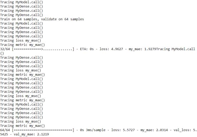
keras.backend.clear_session()
np.random.seed(42)
tf.random.set_seed(42)

model = MyModel(dynamic=True)###############
model.compile(loss=my_mse, optimizer="nadam", metrics=[my_mae])
# Not the custom code will be called at each iteration. 
# Let's fit, validate and evaluate with tiny datasets to avoid getting too much output:
model.fit(X_train_scaled[:64], y_train[:64], epochs=1,
          validation_data=(X_valid_scaled[:64], y_valid[:64]), verbose=0)
model.evaluate(X_test_scaled[:64], y_test[:64], verbose=1)

     If your custom model or layer will always be dynamic, you can instead call the base class’s constructor with dynamic=True:

class MyLayer(keras.layers.Layer):
    def __init__(self, units, **kwargs):
        super().__init__(dynamic=True, **kwargs)
        [...]

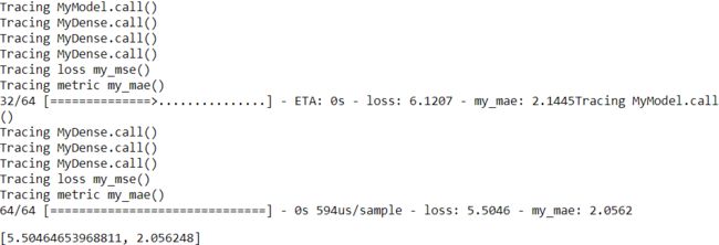
Alternatively, you can compile a model with run_eagerly=True:

keras.backend.clear_session()
np.random.seed(42)
tf.random.set_seed(42)

model = MyModel()
model.compile(loss=my_mse, optimizer="nadam", metrics=[my_mae], run_eagerly=True)###
model.fit(X_train_scaled[:64], y_train[:64], epochs=1,
          validation_data=(X_valid_scaled[:64], y_valid[:64]), verbose=1)
model.evaluate(X_test_scaled[:64], y_test[:64], verbose=1)

     Now you know how TF Functions handle polymorphism (with multiple concrete functions), how graphs are automatically generated using AutoGraph and tracing, what graphs look like, how to explore their symbolic operations and tensors, how to
handle variables and resources, and how to use TF Functions with tf.keras. TensorFlow

Custom Optimizers

Defining custom optimizers is not very common, but in case you are one of the happy few who gets to write one, here is an example:https://blog.csdn.net/Linli522362242/article/details/106982127

class MyMomentumOptimizer( keras.optimizers.Optimizer ):
    def __init__(self, learning_rate=0.001, momentum=0.9, name="MyMomentumOptimizer", **kwargs):
        """Call super().__init__() and use _set_hyper() to store hyperparameters"""
        super().__init__(name, **kwargs)
        self._set_hyper("learning_rate", kwargs.get("lr", learning_rate))#handle lr=learning rate
        #`decay` is included for backward compatibility to allow time inverse decay of learning rate.
        self._set_hyper("decay", self._initial_decay)
        self._set_hyper("momentum", momentum)
        
    def _create_slots(self, var_list):#为每个待更新变量创建用于计算的关联变量
        """For each model variable, create the "optimizer variable" associated with it.
        TensorFlow calls these optimizer variables "slots".
        For momentum optimization, we need one momentum slot per model variable.
        """
        for var in var_list:
            self.add_slot(var, "momentum")
            
    @tf.function
    def _resource_apply_dense(self, grad, var):
        """Update the slots and perform one optimization step for one model variable
        """
        var_dtype = var.dtype.base_dtype    ######
        lr_t = self._decayed_lr(var_dtype) # handle_learning rate decay
        momentum_var = self.get_slot(var, "momentum")
        momentum_hyper = self._get_hyper("momentum", var_dtype)
        #similar to Ada max
        # m <--  m*b - (1-b)*grad
        momentum_var.assign( momentum_var * momentum_hyper - (1.-momentum_hyper)*grad )
        var.assign_add( momentum_var*lr_t )
        
    def _resource_apply_sparse(self, grad, var):
        raise NotImplementedError
    
    def get_config(self):
        base_config = super().get_config()
        return {
            **base_config,
            "learning_rate": self._serialize_hyperparameter("learning_rate"),
            "decay": self._serialize_hyperparameter("decay"),
            "momentum": self._serialize_hyperparameter("momentum"),
        }

keras.backend.clear_session()
np.random.seed(42)
tf.random.set_seed(42)

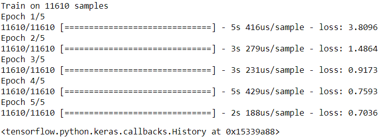
model = keras.models.Sequential([keras.layers.Dense(1, input_shape=[8])])
model.compile(loss="mse", optimizer=MyMomentumOptimizer())
model.fit(X_train_scaled, y_train, epochs=5)

12. Implement a custom layer that performs Layer Normalization (we will use this type of layer in Chapter 15):

     a. The build() method should define two trainable weights α and β, both of shape input_shape[-1:] and data type tf.float32. α should be initialized with 1s, and β with 0s.

     b. The call() method should compute the mean μ and standard deviation σ of each instance’s features. For this, you can use tf.nn.moments(inputs, axes=-1, keepdims=True), which returns the mean μ and the variance of all instances (compute the square root of the variance to get the standard deviation). Then the function should compute and return α⊗(X - μ)/(σ + ε) +β, where ⊗ represents itemwise multiplication (*) and ε is a smoothing term (small constant to avoid division by zero, e.g., 0.001).

 

In this algorithm:

•  is the vector of input means, evaluated over the whole mini-batch B (it contains one mean (average to all features) per input).
•  is the vector of input standard deviations, also evaluated over the whole minibatch B(it contains one standard deviation per input).
•  is the number of instances in the mini-batch.
•  is the vector of zero-centered and normalized inputs for instance i.
• ε is a tiny number that avoids division by zero (typically ). This is called a smoothing term.
• γ is the output scale parameter vector for the layer (it contains one scale parameter per input feature).
• ⊗ represents element-wise multiplication逐元素乘法 (each input is multiplied by its corresponding output scale parameter γ).
• β is the output shift (offset) parameter vector for the layer (it contains one offset parameter per input). Each input is offset by its corresponding shift parameter.
•  is the output of the BN(Batch Normalization) operation. It is a rescaled and shifted version of the inputs.

class LayerNormalization(keras.layers.Layer):
    def __init__(self, eps=0.001, **kwargs):
        super().__init__(**kwargs)
        self.eps = eps
    
    def build(self, batch_input_shape):
        self.alpha = self.add_weight(
            name="alpha", shape=batch_input_shape[-1:],# last element in batch_input_shape(batches, features)
            initializer="ones"
        )                                              # batch_input_shape.shape returns (11610, 8)    
        self.beta = self.add_weight(                   # batch_input_shape[-1] returns 8
            name="beta", shape=batch_input_shape[-1:], # batch_input_shape[-1:] returns (8,)
            initializer = "zeros"
        )

        super().build(batch_input_shape) #must be at the end
    
    # compute the mean μ and standard deviation σ of each instance’s features
    def call(self, X):                    #OR axes=1
        mean, variance = tf.nn.moments(X, axes=-1, keepdims=True)  # mean.shape return(11610, 1)
        #α⊗(X - μ)/(σ + ε) +β
        return self.alpha * (X-mean) / (tf.sqrt(variance+self.eps)) + self.beta
    
    #you can remove it since tf.keras automatically infers the output shape
    def compute_output_shape(self, batch_input_shape):
        return batch_input_shape
    
    def get_config(self):
        base_config = super().get_config()
        return {**base_config, "eps": self.eps}

Note that making ε a hyperparameter (eps) was not compulsory. Also note that it's preferable to compute tf.sqrt(variance + self.eps) rather than tf.sqrt(variance) + self.eps. Indeed, the derivative of sqrt(z) is undefined when z=0### 0.5*1/(z)^0.5 ###, so training will bomb whenever the variance vector has at least one component equal to 0. Adding ε within the square root guarantees that this will never happen. 

c. Ensure that your custom layer produces the same (or very nearly the same) output as the keras.layers.LayerNormalization layer.

Let's create one instance of each class, apply them to some data (e.g., the training set), and ensure that the difference is negligeable.

X = X_train.astype(np.float32) #since tensorflow uses float.32

custom_layer_norm = LayerNormalization()
keras_layer_norm = keras.layers.LayerNormalization()

tf.reduce_mean(keras.losses.mean_absolute_error(
        keras_layer_norm(X), custom_layer_norm(X)
))

#equal to
#tf.reduce_mean(np.abs(
#        keras_layer_norm(X)- custom_layer_norm(X)
#))

Yep, that's close enough. To be extra sure, let's make alpha and beta completely random and compare again:

random_alpha = np.random.rand(X.shape[-1])
random_beta = np.random.rand(X.shape[-1])

custom_layer_norm.set_weights([random_alpha, random_beta]) # since 1 or 0 is not random
keras_layer_norm.set_weights([random_alpha, random_beta])

tf.reduce_mean(keras.losses.mean_absolute_error(
    keras_layer_norm(X), custom_layer_norm(X)
))

custom_layer_norm.weights

random_alpha

keras_layer_norm.weights

13. Train a model using a custom training loop to tackle the Fashion MNIST dataset(see Chapter 10).

a. Display the epoch, iteration, mean training loss, and mean accuracy over each epoch (updated at each iteration), as well as the validation loss and accuracy at the end of each epoch.
 

from tensorflow import keras
import numpy as np
import tensorflow as tf

(X_train_full, y_train_full), (X_test, y_test) = keras.datasets.fashion_mnist.load_data()
## since numpy default uses np.float64, tensor uses np.float32; colour is between 1~255
X_train_full = X_train_full.astype(np.float32) / 255. 
X_valid, X_train = X_train_full[:5000], X_train_full[5000:]
y_valid, y_train = y_train_full[:5000], y_train_full[5000:]
X_test = X_test.astype(np.float32) / 255.

keras.backend.clear_session()
np.random.seed(42)
tf.random.set_seed(42)

model = keras.models.Sequential([
    keras.layers.Flatten( input_shape=[28,28]),
    keras.layers.Dense(100, activation='relu'),
    keras.layers.Dense(10, activation="softmax"), # use softmax for classification
])

n_epochs = 5
batch_size = 32
n_steps = len(X_train) // batch_size
optimizer = keras.optimizers.Nadam(lr=0.01)

loss_fn = keras.losses.sparse_categorical_crossentropy
mean_loss = keras.metrics.Mean()

metrics = [keras.metrics.SparseCategoricalAccuracy()]

from tqdm.notebook import trange
from collections import OrderedDict

def random_batch(X, y, batch_size=32):
    idx = np.random.randint( len(X), size=batch_size)# selection
    return X[idx], y[idx]

with trange(1, n_epochs + 1, desc="All epochs") as epochs:
    for epoch in epochs:
        
        with trange(1, n_steps+1, desc="Epoch {}/{}".format(epoch, n_epochs)) as steps:
            for step in steps:
                
                X_batch, y_batch = random_batch(X_train, y_train)
                
                with tf.GradientTape() as tape:
                    # make a prediction for one batch (using the model as a function
                    y_pred = model(X_batch)
                    # keras.losses.sparse_categorical_crossentropy
                    main_loss = tf.reduce_mean(loss_fn(y_batch, y_pred))
                    # model.losses: there is one "regularization loss" per layer)
                    # The regularization losses are already reduced to a single scalar each
                    loss = tf.add_n( [main_loss]+model.losses )
                    
                # compute the gradient of the loss with regard to each trainable variable    
                gradients = tape.gradient(loss, model.trainable_variables)
                optimizer.apply_gradients(zip(gradients, model.trainable_variables))
               
            
                ######################## constraint ########################
                # If you add weight constraints to your model (e.g., by setting kernel_constraint 
                # or bias_constraint when creating a layer), you should update the training loop to
                # apply these constraints just after apply_gradients():
                for variable in model.variables:
                    if variable.constraint is not None:
                        variable.assign(variable.constraint(variable))
                        
                status = OrderedDict() 
                mean_loss(loss) # mean_loss = keras.metrics.Mean()
                status["loss"] = mean_loss.result().numpy()
                # metrics = [keras.metrics.SparseCategoricalAccuracy()] 
                for metric in metrics:
                    metric(y_batch, y_pred)
                    status[metric.name] = metric.result().numpy()
                steps.set_postfix(status)
                
            # end step
            y_pred =model(X_valid)
            status['val_loss'] = np.mean(loss_fn(y_valid, y_pred))
            status['val_accuracy'] = np.mean(keras.metrics.sparse_categorical_accuracy(
                                                 tf.constant(y_valid, dtype=np.float32), 
                                                 y_pred
                                                )        
                                            )
            steps.set_postfix(status)
        # At the end of each epoch, we display the status bar again to make it look complete
        # and to print a line feed, and we reset the states of the mean loss and the metrics.
        for metric in [mean_loss] + metrics:
            metric.reset_states()

 

b. Try using a different optimizer with a different learning rate for the upper layers and the lower layers.

keras.backend.clear_session()
np.random.seed(42)
tf.random.set_seed(42)


lower_layers = keras.models.Sequential([
    keras.layers.Flatten(input_shape=[28,28]),
    keras.layers.Dense(100, activation="relu"),
])

upper_layers = keras.models.Sequential([
    keras.layers.Dense(10, activation="softmax"),
])

model = keras.models.Sequential([
    lower_layers, upper_layers
])


lower_optimizer = keras.optimizers.SGD(lr=1e-4)
upper_optimizer = keras.optimizers.Nadam(lr=1e-3)
                                         
batch_size = 32
n_steps = len(X_train) // batch_size
                                         
loss_fn = keras.losses.sparse_categorical_crossentropy
mean_loss = keras.metrics.Mean()
metrics = [keras.metrics.SparseCategoricalAccuracy()]


with trange(1, n_epochs + 1, desc="All epochs") as epochs:
    for epoch in epochs:
        
        with trange(1, n_steps+1, desc="Epoch {}/{}".format(epoch, n_epochs)) as steps:
            for step in steps:
                
                X_batch, y_batch = random_batch(X_train, y_train)
                # call gradient() more than once
                with tf.GradientTape(persistent=True) as tape:
                    y_pred = model(X_batch)
                    main_loss = tf.reduce_mean(loss_fn(y_batch, y_pred))
                    loss = tf.add_n([main_loss] + model.losses)
                
                for layers, optimizer in ((lower_layers, lower_optimizer),
                                          (upper_layers, upper_optimizer)):
                    gradients = tape.gradient(loss, layers.trainable_variables)
                    optimizer.apply_gradients(zip(gradients, layers.trainable_variables))
                
                del tape

                ######################## constraint ########################
                # If you add weight constraints to your model (e.g., by setting kernel_constraint 
                # or bias_constraint when creating a layer), you should update the training loop to
                # apply these constraints just after apply_gradients():
                for variable in model.variables:
                    if variable.constraint is not None:
                        variable.assign(variable.constraint(variable))
                        
                status = OrderedDict()
                mean_loss(loss)
                status["loss"] = mean_loss.result().numpy()
                for metric in metrics:
                    metric(y_batch, y_pred)
                    status[metric.name] = metric.result().numpy()
                steps.set_postfix(status)
                
            y_pred = model(X_valid)
            status["val_loss"] = np.mean(loss_fn(y_valid, y_pred))
            status['val_accuracy'] = np.mean(keras.metrics.sparse_categorical_accuracy(
                                                 tf.constant(y_valid, dtype=np.float32),
                                                 y_pred
                                                )
                                            )
            steps.set_postfix(status)
        for metric in [mean_loss] + metrics:
            metric.reset_states()