CS231n Lecture 2: Image Classification pipeline

Assignment

Image Classification pipeline

• Nearest Classification
• K-Nearest Neighbors(KNN)
• Liner classification

Code Achievement

Working locally

• Installing Anaconda
• Anaconda Virtual environment

Once you have Anaconda installed, it makes sense to create a virtual environment for the course. If you choose not to use a virtual environment, it is up to you to make sure that all dependencies for the code are installed globally on your machine. To set up a virtual environment, run (in a terminal)

conda create -n cs231n python=3.7 anaconda

to create an environment called cs231n.
Then you can find Anaconda Prompt(cs231n) and Jupyter Notebook(cs231n) in your Anaconda FIle.
You may refer to this page for more detailed instructions on managing virtual environments with Anaconda.

Download Dataset

Once you have the starter code , you will need to download the CIFAR-10 dataset. Run the following from the assignment1 directory:

cd cs231n/datasets
./get_datasets.sh

for windows, get dataset from http://www.cs.toronto.edu/~kriz/cifar-10-python.tar.gz ,then unzip to datasets

Start IPython

After you have the CIFAR-10 data, you should start the IPython notebook server from the assignment1 directory, with the jupyter notebook command.

Code Achievement

import modules

# Run some setup code for this notebook.

import random
import numpy as np
from cs231n.data_utils import load_CIFAR10
import matplotlib.pyplot as plt

# This is a bit of magic to make matplotlib figures appear inline in the notebook
# rather than in a new window.
%matplotlib inline
plt.rcParams['figure.figsize'] = (10.0, 8.0) # set default size of plots
plt.rcParams['image.interpolation'] = 'nearest'
plt.rcParams['image.cmap'] = 'gray'

# Some more magic so that the notebook will reload external python modules;
# see http://stackoverflow.com/questions/1907993/autoreload-of-modules-in-ipython
%load_ext autoreload
%autoreload 2

load_CIFAR10 in data_utils.py

def load_CIFAR10(ROOT): 
    """ load all of cifar """
    xs = []
    ys = []
    for b in range(1,6):
        f = os.path.join(ROOT, 'data_batch_%d' % (b, )) #combine to filename
        X, Y = load_CIFAR_batch(f) # read f
        xs.append(X)
        ys.append(Y)
    Xtr = np.concatenate(xs)
    Ytr = np.concatenate(ys)
    del X, Y
    Xte, Yte = load_CIFAR_batch(os.path.join(ROOT, 'test_batch'))
    return Xtr, Ytr, Xte, Yte

def load_CIFAR_batch(filename):
    """ load single batch of cifar """
    with open(filename, 'rb') as f:
        datadict = load_pickle(f) #read & write in file
        X = datadict['data']
        Y = datadict['labels']
        X = X.reshape(10000, 3, 32, 32).transpose(0,2,3,1).astype("float") #original data type; transpose:change position 0:10000 data num,1:3 channel,2&3:32*32 image size
        Y = np.array(Y)
        return X, Y

Load data

# Load the raw CIFAR-10 data.
cifar10_dir = 'cs231n/datasets/cifar-10-batches-py'#it may be error in windows,you can change '/' to '\\' or use the other way to define the fileload as written below.
#import os
#cifar10_dir = os.path.join("cs231n","datasets","cifar-10-batches-py")


# Cleaning up variables to prevent loading data multiple times (which may cause memory issue)
try:
   del X_train, y_train
   del X_test, y_test
   print('Clear previously loaded data.')
except:
   pass

X_train, y_train, X_test, y_test = load_CIFAR10(cifar10_dir)

# As a sanity check, we print out the size of the training and test data.
print('Training data shape: ', X_train.shape)
print('Training labels shape: ', y_train.shape)
print('Test data shape: ', X_test.shape)
print('Test labels shape: ', y_test.shape)

out:
Training data shape:  (50000, 32, 32, 3)
Training labels shape:  (50000,)
Test data shape:  (10000, 32, 32, 3)
Test labels shape:  (10000,)

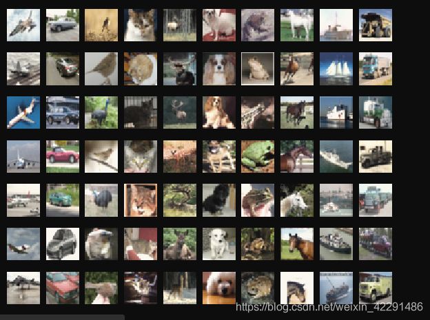
# Visualize some examples from the dataset.
# We show a few examples of training images from each class.
classes = ['plane', 'car', 'bird', 'cat', 'deer', 'dog', 'frog', 'horse', 'ship', 'truck']
num_classes = len(classes)
samples_per_class = 7
for y, cls in enumerate(classes):
    idxs = np.flatnonzero(y_train == y)
    idxs = np.random.choice(idxs, samples_per_class, replace=False)
    for i, idx in enumerate(idxs):
        plt_idx = i * num_classes + y + 1
        plt.subplot(samples_per_class, num_classes, plt_idx)
        plt.imshow(X_train[idx].astype('uint8'))
        plt.axis('off')
        if i == 0:
            plt.title(cls)
plt.show()

# Subsample the data for more efficient code execution in this exercise
num_training = 5000
mask = list(range(num_training))
X_train = X_train[mask]
y_train = y_train[mask]

num_test = 500
mask = list(range(num_test))
X_test = X_test[mask]
y_test = y_test[mask]

# Reshape the image data into rows
X_train = np.reshape(X_train, (X_train.shape[0], -1))
X_test = np.reshape(X_test, (X_test.shape[0], -1))
print(X_train.shape, X_test.shape)

out
(5000, 3072) (500, 3072)

KNN

from cs231n.classifiers import KNearestNeighbor

# Create a kNN classifier instance. 
# Remember that training a kNN classifier is a noop: 
# the Classifier simply remembers the data and does no further processing 
classifier = KNearestNeighbor()
classifier.train(X_train, y_train)

We would now like to classify the test data with the kNN classifier. Recall that we can break down this process into two steps:

First we must compute the distances between all test examples and all train examples.
Given these distances, for each test example we find the k nearest examples and have them vote for the label
Lets begin with computing the distance matrix between all training and test examples. For example, if there are Ntr training examples and Nte test examples, this stage should result in a Nte x Ntr matrix where each element (i,j) is the distance between the i-th test and j-th train example.

Note: For the three distance computations that we require you to implement in this notebook, you may not use the np.linalg.norm() function that numpy provides.

First, open cs231n/classifiers/k_nearest_neighbor.py and implement the function compute_distances_two_loops that uses a (very inefficient) double loop over all pairs of (test, train) examples and computes the distance matrix one element at a time.

# Open cs231n/classifiers/k_nearest_neighbor.py and implement
# compute_distances_two_loops.

# Test your implementation:
dists = classifier.compute_distances_two_loops(X_test)
print(dists.shape)

k_nearest_neighbor.py

from builtins import range
from builtins import object
import numpy as np
from past.builtins import xrange #if the error "No module named 'past'" happened, install 'future' module by "pip install future"
def compute_distances_two_loops(self, X):
        """
        Compute the distance between each test point in X and each training point
        in self.X_train using a nested loop over both the training data and the
        test data.

        Inputs:
        - X: A numpy array of shape (num_test, D) containing test data.

        Returns:
        - dists: A numpy array of shape (num_test, num_train) where dists[i, j]
          is the Euclidean(L2) distance between the ith test point and the jth training
          point.
        """
        num_test = X.shape[0]
        num_train = self.X_train.shape[0]
        dists = np.zeros((num_test, num_train))
        for i in range(num_test):
            for j in range(num_train):
                #####################################################################
                # TODO:                                                             #
                # Compute the l2 distance between the ith test point and the jth    #
                # training point, and store the result in dists[i, j]. You should   #
                # not use a loop over dimension, nor use np.linalg.norm().          #
                #####################################################################
                # *****START OF YOUR CODE (DO NOT DELETE/MODIFY THIS LINE)*****
				dists[i,j] =  np.sqrt( sum( np.square(X[i,:] - self.X_train[j,:])))#this is my answer
                pass

                # *****END OF YOUR CODE (DO NOT DELETE/MODIFY THIS LINE)*****
        return dists

# We can visualize the distance matrix: each row is a single test example and
# its distances to training examples
plt.imshow(dists, interpolation='none')
plt.show()

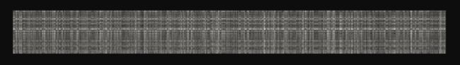
Inline Question 1

Notice the structured patterns in the distance matrix, where some rows or columns are visible brighter. (Note that with the default color scheme black indicates low distances while white indicates high distances.)

What in the data is the cause behind the distinctly bright rows?
What causes the columns?
Y?????????:  
- Cause each row is a single test example and its distance to training example, darker pixels mean the examples are more familiars to some of the training data and the white pixels mean on the contrary.
- However, bright rows exist, which means theses test examples are much less similar with training data. Maybe the test examples belong none of these ten classes or maybe their pixel value are quite different with training data because of noise, background or something, which connected to our algorithm robustness.

result

k_nearest_neighbor,py

def predict_labels(self, dists, k=1):
  		 """
        Given a matrix of distances between test points and training points,
        predict a label for each test point.

        Inputs:
        - dists: A numpy array of shape (num_test, num_train) where dists[i, j]
          gives the distance betwen the ith test point and the jth training point.

        Returns:
        - y: A numpy array of shape (num_test,) containing predicted labels for the
          test data, where y[i] is the predicted label for the test point X[i].
        """
        num_test = dists.shape[0]
        y_pred = np.zeros(num_test)
        for i in range(num_test):
            # A list of length k storing the labels of the k nearest neighbors to
            # the ith test point.
            closest_y = []
            #########################################################################
            # TODO:                                                                 #
            # Use the distance matrix to find the k nearest neighbors of the ith    #
            # testing point, and use self.y_train to find the labels of these       #
            # neighbors. Store these labels in closest_y.                           #
            # Hint: Look up the function numpy.argsort. 
            # argsort: Returns the indices that would sort an array.  return the items position after they were sort.                          #
            #########################################################################
            # *****START OF YOUR CODE (DO NOT DELETE/MODIFY THIS LINE)*****
            index_rank = np.argsort(dists[i,:])#rank dist from low to high
            index_k = index_rank[0:k]# selcet the kth dist
            closest_y = self.y_train[index_k]# find the corresponding labels
            pass

            # *****END OF YOUR CODE (DO NOT DELETE/MODIFY THIS LINE)*****
            #########################################################################
            # TODO:                                                                 #
            # Now that you have found the labels of the k nearest neighbors, you    #
            # need to find the most common label in the list closest_y of labels.   #
            # Store this label in y_pred[i]. Break ties by choosing the smaller     #
            # label.                                                                #
            #########################################################################
            # *****START OF YOUR CODE (DO NOT DELETE/MODIFY THIS LINE)*****
			sort = sorted(Counter(closest_y).items(),key=lambda item:item[1],reverse = True)# need "from collections import Counter"
            y_pred[i] = sort[0][0]
            pass

            # *****END OF YOUR CODE (DO NOT DELETE/MODIFY THIS LINE)*****

        return y_pred

# Now implement the function predict_labels and run the code below:
# We use k = 1 (which is Nearest Neighbor).
y_test_pred = classifier.predict_labels(dists, k=1)

# Compute and print the fraction of correctly predicted examples
num_correct = np.sum(y_test_pred == y_test)
accuracy = float(num_correct) / num_test
print('Got %d / %d correct => accuracy: %f' % (num_correct, num_test, accuracy))

out: Got 137 / 500 correct => accuracy: 0.274000

You should expect to see approximately 27% accuracy. Now lets try out a larger k, say k = 5:

y_test_pred = classifier.predict_labels(dists, k=5)
num_correct = np.sum(y_test_pred == y_test)
accuracy = float(num_correct) / num_test
print('Got %d / %d correct => accuracy: %f' % (num_correct, num_test, accuracy))

out: Got 137 / 500 correct => accuracy: 0.290000

You should expect to see a slightly better performance than with k = 1.

I recommend this answer.

optimization

iteration

# Now lets speed up distance matrix computation by using partial vectorization
# with one loop. Implement the function compute_distances_one_loop and run the
# code below:
dists_one = classifier.compute_distances_one_loop(X_test)

# To ensure that our vectorized implementation is correct, we make sure that it
# agrees with the naive implementation. There are many ways to decide whether
# two matrices are similar; one of the simplest is the Frobenius norm. In case
# you haven't seen it before, the Frobenius norm of two matrices is the square
# root of the squared sum of differences of all elements; in other words, reshape
# the matrices into vectors and compute the Euclidean distance between them.
difference = np.linalg.norm(dists - dists_one, ord='fro')
print('One loop difference was: %f' % (difference, ))
if difference < 0.001:
    print('Good! The distance matrices are the same')
else:
    print('Uh-oh! The distance matrices are different')

k_nearest_neighbor,py

def compute_distances_one_loop(self, X):
        """
        Compute the distance between each test point in X and each training point
        in self.X_train using a single loop over the test data.

        Input / Output: Same as compute_distances_two_loops
        """
        num_test = X.shape[0]
        num_train = self.X_train.shape[0]
        dists = np.zeros((num_test, num_train))
        for i in range(num_test):
            #######################################################################
            # TODO:                                                               #
            # Compute the l2 distance between the ith test point and all training #
            # points, and store the result in dists[i, :].                        #
            # Do not use np.linalg.norm().                                        #
            #######################################################################
            # *****START OF YOUR CODE (DO NOT DELETE/MODIFY THIS LINE)*****
			dists[i,:] =  np.sqrt(np.sum(np.square(X[i,:] - self.X_train),axis =1))
			#axis =1 means sum horizontally
            pass

            # *****END OF YOUR CODE (DO NOT DELETE/MODIFY THIS LINE)*****
        return dists

out:
One loop difference was: 0.000000
Good! The distance matrices are the same

# Now implement the fully vectorized version inside compute_distances_no_loops
# and run the code
dists_two = classifier.compute_distances_no_loops(X_test)

# check that the distance matrix agrees with the one we computed before:
difference = np.linalg.norm(dists - dists_two, ord='fro')
print('No loop difference was: %f' % (difference, ))
if difference < 0.001:
    print('Good! The distance matrices are the same')
else:
    print('Uh-oh! The distance matrices are different')

out:
One loop difference was: 0.000000
Good! The distance matrices are the same

here’s some messages about broadcast.

def compute_distances_no_loops(self, X):
        """
        Compute the distance between each test point in X and each training point
        in self.X_train using no explicit loops.

        Input / Output: Same as compute_distances_two_loops
        """
        num_test = X.shape[0]
        num_train = self.X_train.shape[0]
        dists = np.zeros((num_test, num_train))
        #########################################################################
        # TODO:                                                                 #
        # Compute the l2 distance between all test points and all training      #
        # points without using any explicit loops, and store the result in      #
        # dists.                                                                #
        #                                                                       #
        # You should implement this function using only basic array operations; #
        # in particular you should not use functions from scipy,                #
        # nor use np.linalg.norm().                                             #
        #                                                                       #
        # HINT: Try to formulate the l2 distance using matrix multiplication    #
        #       and two broadcast sums.                                         #
        #########################################################################
        # *****START OF YOUR CODE (DO NOT DELETE/MODIFY THIS LINE)*****
        dists += np.sum(self.X_train ** 2, axis=1).reshape(1, num_train) #1*5000，the first broadcast
        dists += np.sum(X ** 2, axis=1).reshape(num_test,1) #500*1，the second broadcast
        dists -= 2 * np.dot(X, self.X_train.T) #500*5000
        dists = np.sqrt(dists)


        pass

        # *****END OF YOUR CODE (DO NOT DELETE/MODIFY THIS LINE)*****
        return dists

more detials

# Let's compare how fast the implementations are
def time_function(f, *args):
    """
    Call a function f with args and return the time (in seconds) that it took to execute.
    """
    import time
    tic = time.time()
    f(*args)
    toc = time.time()
    return toc - tic

two_loop_time = time_function(classifier.compute_distances_two_loops, X_test)
print('Two loop version took %f seconds' % two_loop_time)

one_loop_time = time_function(classifier.compute_distances_one_loop, X_test)
print('One loop version took %f seconds' % one_loop_time)

no_loop_time = time_function(classifier.compute_distances_no_loops, X_test)
print('No loop version took %f seconds' % no_loop_time)

# You should see significantly faster performance with the fully vectorized implementation!

# NOTE: depending on what machine you're using, 
# you might not see a speedup when you go from two loops to one loop, 
# and might even see a slow-down.

out:
Two loop version took 2330.480827 seconds
One loop version took 129.882184 seconds
No loop version took 0.886452 seconds

Cross-validation

We have implemented the k-Nearest Neighbor classifier but we set the value k = 5 arbitrarily. We will now determine the best value of this hyperparameter with cross-validation.

num_folds = 5
k_choices = [1, 3, 5, 8, 10, 12, 15, 20, 50, 100]

X_train_folds = []
y_train_folds = []
################################################################################
# TODO:                                                                        #
# Split up the training data into folds. After splitting, X_train_folds and    #
# y_train_folds should each be lists of length num_folds, where                #
# y_train_folds[i] is the label vector for the points in X_train_folds[i].     #
# Hint: Look up the numpy array_split function.                                #
################################################################################
# *****START OF YOUR CODE (DO NOT DELETE/MODIFY THIS LINE)*****
X_train_folds = np.vsplit(X_train,num_folds)
y_train_folds = np.split(y_train,num_folds)
pass

# *****END OF YOUR CODE (DO NOT DELETE/MODIFY THIS LINE)*****

# A dictionary holding the accuracies for different values of k that we find
# when running cross-validation. After running cross-validation,
# k_to_accuracies[k] should be a list of length num_folds giving the different
# accuracy values that we found when using that value of k.
k_to_accuracies = {}


################################################################################
# TODO:                                                                        #
# Perform k-fold cross validation to find the best value of k. For each        #
# possible value of k, run the k-nearest-neighbor algorithm num_folds times,   #
# where in each case you use all but one of the folds as training data and the #
# last fold as a validation set. Store the accuracies for all fold and all     #
# values of k in the k_to_accuracies dictionary.                               #
################################################################################
# *****START OF YOUR CODE (DO NOT DELETE/MODIFY THIS LINE)*****
for k in k_choices:
    accuracies = []
    for i in range(num_folds):

        x_train_val = X_train_folds[i]
        y_train_val = y_train_folds[i]
        #del X_train_folds[i]
        #del y_train_folds[i]
        xtrain_list = np.vstack(X_train_folds[0:i] + X_train_folds[i+1:])
        ytrain_list = np.hstack(y_train_folds[0:i] + y_train_folds[i+1:])

        classifier.train(xtrain_list,ytrain_list)
        dists = classifier.compute_distances_no_loops(x_train_val)
        y_test_pred = classifier.predict_labels(dists, k)
        num_correct = np.sum(y_test_pred == y_train_val)
        accuracy = float(num_correct) /  y_train_val.shape[0]
        accuracies.append(accuracy)
    k_to_accuracies[k] = accuracies
pass

# *****END OF YOUR CODE (DO NOT DELETE/MODIFY THIS LINE)*****

# Print out the computed accuracies
for k in sorted(k_to_accuracies):
    for accuracy in k_to_accuracies[k]:
        print('k = %d, accuracy = %f' % (k, accuracy))

# plot the raw observations
for k in k_choices:
   accuracies = k_to_accuracies[k]
   plt.scatter([k] * len(accuracies), accuracies)

# plot the trend line with error bars that correspond to standard deviation
accuracies_mean = np.array([np.mean(v) for k,v in sorted(k_to_accuracies.items())])
accuracies_std = np.array([np.std(v) for k,v in sorted(k_to_accuracies.items())])
plt.errorbar(k_choices, accuracies_mean, yerr=accuracies_std)
plt.title('Cross-validation on k')
plt.xlabel('k')
plt.ylabel('Cross-validation accuracy')
plt.show()

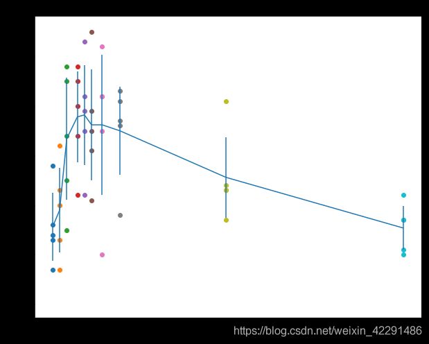
# Based on the cross-validation results above, choose the best value for k,   
# retrain the classifier using all the training data, and test it on the test
# data. You should be able to get above 28% accuracy on the test data.

temp = accuracies_mean.tolist()
best_kth = temp.index(max(temp))
best_k = k_choices[best_kth]

print(best_k)


classifier = KNearestNeighbor()
classifier.train(X_train, y_train)
y_test_pred = classifier.predict(X_test, k=best_k)

# Compute and display the accuracy
num_correct = np.sum(y_test_pred == y_test)
accuracy = float(num_correct) / num_test
print('Got %d / %d correct => accuracy: %f' % (num_correct, num_test, accuracy))

out:
10
Got 144 / 500 correct => accuracy: 0.288000

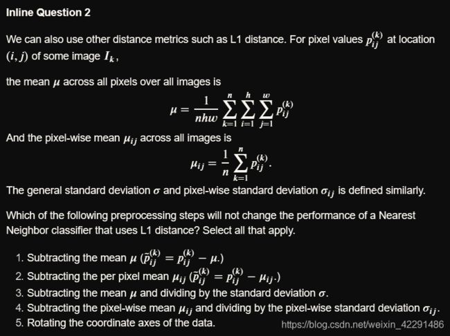
Inline Question 3

Which of the following statements about  ? -Nearest Neighbor ( ? -NN) are true in a classification setting, and for all  ? ? Select all that apply.

The decision boundary of the k-NN classifier is linear.
The training error of a 1-NN will always be lower than that of 5-NN.
The test error of a 1-NN will always be lower than that of a 5-NN.
The time needed to classify a test example with the k-NN classifier grows with the size of the training set.
None of the above.
Y?????????: 4
Y??????????????:
1. irregular shape
2. 5-NN has more robustness and lower train error
3. it has uncertainty
4. in test process all datas are used including traing data, so it need more time  with larger size of the trainging set.