kmeans算法
文章目录
- 1、概述
-
- 1.1 无监督学习与聚类算法
- 1.2 sklearn中的聚类算法
- 2、KMeans
-
- 2.1 KMeans是如何工作的?
- 2.2 簇内误差平方和的定义和解惑
- 3、sklearn.cluster.KMeans
-
- 3.1 重要参数n_clusters
- 3.2 聚类算法的模型评估指标
-
- 3.2.1当真实标签已知时
- 3.2.2 当真实标签未知时:轮廓系数
- 3.3案例:基于轮廓系数来选择n_clusters
- 3.4 重要参数init & random_state & n_init:初始质心怎么放好?
- 3.5 重要参数max_iter& tol:让迭代停下来
- 3.6 重要属性与重要接口
- 3.7函数cluster.k_means
- 4、案例:聚类算法用于降维,KMeans的矢量量化应用
1、概述
1.1 无监督学习与聚类算法
决策树、随机森林、逻辑回归属于“有监督学习”,即模型在训练的时候,不仅特征矩阵X,还需要真实标签y。机器学习中,还有“无监督学习”,无监督的算法在训练的时候只需要特征矩阵X,不需要标签。PCA降维算法就是无监督学习中的一种,聚类算法,也是无监督学习的代表算法之一。
聚类算法又叫做“无监督分类”,其目的是将数据划分成有意义或有用的组(或簇)。比如在商业中,如果我们手头有大量的当前和潜在客户的信息,我们可以使用聚类将客户划分为若干组,以便进一步分析和开展营销活动,最有名的客户价值判断模型RFM,就常常和聚类分析共同使用。再比如,聚类可以用于降维和矢量量化(vector quantization),可以将高维特征压缩到一列当中,常常用于图像,声音,视频等非结构化数据,可以大幅度压缩
数据量。
有监督学习和无监督学习的区别:

1.2 sklearn中的聚类算法
聚类算法在sklearn中有两种表现形式,一种是类(和我们目前为止学过的分类算法以及数据预处理方法们都一样),需要实例化,训练并使用接口和属性来调用结果。另一种是函数(function),只需要输入特征矩阵和超参数,即可返回聚类的结果和各种指标。

2、KMeans
2.1 KMeans是如何工作的?
作为聚类算法的典型代表,KMeans可以说是最简单的聚类算法没有之一,那它是怎么完成聚类的呢?
在KMeans算法中,簇的个数K是一个超参数,需要我们人为输入来确定。KMeans的核心任务就是根据我们设定好的K,找出K个最优的质心,并将离这些质心最近的数据分别分配到这些质心代表的簇中去。具体过程可以总结如下:

那什么情况下,质心的位置会不再变化呢?当我们找到一个质心,在每次迭代中被分配到这个质心上的样本都是一致的,即每次新生成的簇都是一致的,所有的样本点都不会再从一个簇转移到另一个簇,质心就不会变化了。这个过程在可以由下图来显示,我们规定,将数据分为4簇(K=4),其中白色X代表质心的置:
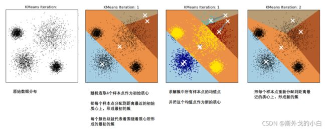
第六次迭代之后,基本上质心的位置就不再改变了,生成的簇也变得稳定。此时我们的聚类就完成了,我们可以明显看出,KMeans按照数据的分布,将数据聚集成了我们规定的4类,接下来我们就可以按照我们的业务需求或者算法需求,对这四类数据进行不同的处理。
2.2 簇内误差平方和的定义和解惑
聚类算法聚出的类有什么含义呢?这些类有什么样的性质?我们认为,被分在同一个簇中的数据是有相似性的,而不同簇中的数据是不同的,当聚类完毕之后,我们就要分别去研究每个簇中的样本都有什么样的性质,从而根据业
务需求制定不同的商业或者科技策略。我们追求“组内差异小,组间差异大”。聚类算法也是同样的目的,我们追求“簇内差异小,簇外差异大”。而这个“差异“,由样本点到其所在簇的质心的距离来衡量。
对于一个簇来说,所有样本点到质心的距离之和越小,我们就认为这个簇中的样本越相似,簇内差异就越小。而距离的衡量方法有多种,令 表示簇中的一个样本点, 表示该簇中的质心,n表示每个样本点中的特征数目,i表示组
成点 的每个特征,则该样本点到质心的距离可以由以下距离来度量:

如我们采用欧几里得距离,则一个簇中所有样本点到质心的距离的平方和为:

m为一个簇中样本的个数,j是每个样本的编号。这个公式被称为簇内平方和(cluster Sum of Square),又叫做Inertia。而将一个数据集中的所有簇的簇内平方和相加,就得到了整体平方和(Total Cluster Sum of Square),又叫做total inertia。Total Inertia越小,代表着每个簇内样本越相似,聚类的效果就越好。因此KMeans追求的是,求解能够让Inertia最小化的质心。实际上,在质心不断变化不断迭代的过程中,总体平方和是越来越小的。我们可以使用数学来证明,当整体平方和最小的时候,质心就不再发生变化了。如此,K-Means的求解过程,就变成了一个最优化问题。


而这些组合,都可以由严格的数学证明来推导。在sklearn当中,我们无法选择使用的距离,只能使用欧式距离。因此,我们也无需去担忧这些距离所搭配的质心选择是如何得来的了。
3、sklearn.cluster.KMeans
3.1 重要参数n_clusters
n_clusters是KMeans中的k,表示着我们告诉模型我们要分几类。这是KMeans当中唯一一个必填的参数,默认为8类,但通常我们的聚类结果会是一个小于8的结果。通常,在开始聚类之前,我们并不知道n_clusters究竟是多少,因此我们要对它进行探索。
from sklearn.datasets import make_blobs
from matplotlib import pyplot as plt
from sklearn.cluster import KMeans
from sklearn.metrics import silhouette_samples
from sklearn.metrics import silhouette_score
from sklearn.metrics import calinski_harabasz_score
from time import time

x, y = make_blobs(n_samples=500, n_features=2, centers=4, random_state=1)
#建立一个有二维特征、4个中心范围的样本量为500的数据集
print(x, y)
print(x[:, 0])

fig, ax1 = plt.subplots(1)
#fig是画布,ax1是对象,画1个子图,由于没有定义对象,所以在画布中显示不出任何东西喔
ax1.scatter(x[:, 0], x[:, 1],
            marker='o',  #点的形状
            s=8)        #点的大小

plt.show()

n_clusters = 3
cluster = KMeans(n_clusters=n_clusters, random_state=1).fit(x)

y_pred = cluster.labels_
#print(y_pred)

pre = cluster.fit_predict(x)
#print(pre)

#print(pre == y_pred)

cluster_ = KMeans(n_clusters=n_clusters, random_state=1).fit(x[:200])
y_pred_ = cluster_.predict(x)
#print(y_pred == y_pred_)

centroid = cluster.cluster_centers_
#print(centroid)  #质心
#print(centroid.shape)  #(3, 2)

inertia = cluster.inertia_  #所有点和质心的距离平方和
#print(inertia)  #1903.4503741659219
color = ['red', 'pink', 'orange', 'gray']
fig, ax1 = plt.subplots(1)

for i in range(n_clusters):
    ax1.scatter(x[y_pred == i, 0], x[y_pred == i, 1],
                marker='o',
                s=8,
                c=color[i])
ax1.scatter(centroid[:, 0], centroid[:, 1],
            marker='x',
            s=25,
            c='black')

plt.show()

n_clusters = 4
cluster_1 = KMeans(n_clusters=n_clusters, random_state=1).fit(x)
inertia_ = cluster_1.inertia_
#print(inertia_)  #908.3855684760615

n_clusters = 5
cluster_2 = KMeans(n_clusters=n_clusters, random_state=1).fit(x)
inertia_1 = cluster_2.inertia_
#print(inertia_1)  #811.0170422004205

n_clusters = 6
cluster_3 = KMeans(n_clusters=n_clusters, random_state=1).fit(x)
inertia_2 = cluster_3.inertia_
#print(inertia_2)  #729.924401937258
我们可以看到inertia随着簇的增加而减少,但是inerita具有评估参考性吗?并不是,当簇组件增加的时候,inertia会逐渐减小,当簇的个数和样本个数一致的时候,inertia=0。所以inertia并不能作为评估指标。
3.2 聚类算法的模型评估指标

inertia的缺陷:
(1)它不是有界的。我们只知道,Inertia是越小越好,是0最好,但我们不知道,一个较小的Inertia究竟有没有达到模型的极限,能否继续提高。
(2)它的计算太容易受到特征数目的影响,数据维度很大的时候,Inertia的计算量会陷入维度诅咒之中,计算量会爆炸,不适合用来一次次评估模型。
(3)它会受到超参数K的影响,在我们之前的常识中其实我们已经发现,随着K越大,Inertia注定会越来越小,但这并不代表模型的效果越来越好了
(4)Inertia对数据的分布有假设,它假设数据满足凸分布(即数据在二维平面图像上看起来是一个凸函数的样子),并且它假设数据是各向同性的(isotropic),即是说数据的属性在不同方向上代表着相同的含义。但是现实
中的数据往往不是这样。所以使用Inertia作为评估指标,会让聚类算法在一些细长簇,环形簇,或者不规则形状的流形时表现不佳:

3.2.1当真实标签已知时

3.2.2 当真实标签未知时:轮廓系数
轮廓系数是最常用的聚类算法的评价指标。它是对每个样本来定义的,它能够同时衡量:
1)样本与其自身所在的簇中的其他样本的相似度a,等于样本与同一簇中所有其他点之间的平均距离;
2)样本与其他簇中的样本的相似度b,等于样本与下一个最近的簇中的所有点之间的平均距离.
根据聚类的要求”簇内差异小,簇外差异大“,我们希望b永远大于a,并且大得越多越好。
单个样本的轮廓系数计算为:

这个公式可以被解析为:

很容易理解轮廓系数范围是(-1,1),其中值越接近1表示样本与自己所在的簇中的样本很相似,并且与其他簇中的样本不相似,当样本点与簇外的样本更相似的时候,轮廓系数就为负。当轮廓系数为0时,则代表两个簇中的样本相似度一致,两个簇本应该是一个簇。可以总结为轮廓系数越接近于1越好,负数则表示聚类效果非常差。
在sklearn中,我们使用模块metrics中的类silhouette_score来计算轮廓系数,它返回的是一个数据集中,所有样本的轮廓系数的均值。但我们还有同在metrics模块中的silhouette_sample,它的参数与轮廓系数一致,但返回的是数据集中每个样本自己的轮廓系数。
t0 = time()
print(silhouette_score(x, y_pred)) #0.5882004012129721
t1 = time()
t_1 = t1 - t0

print(t_1)  #0.005017757415771484
print(silhouette_score(x, cluster_1.labels_)) #0.6505186632729437
print(silhouette_score(x, cluster_2.labels_)) #0.5743946554642042
print(silhouette_score(x, cluster_3.labels_)) #0.5141489067073599

print(silhouette_samples(x, y_pred).mean())  #0.58820040121297
print(silhouette_samples(x, y_pred))
#给出每个样本的轮廓系数值
3.2.3 当真实标签未知时:Calinski-Harabaz Index
除了轮廓系数是最常用的,我们还有卡林斯基-哈拉巴斯指数(Calinski-Harabaz Index,简称CHI,也被称为方差比标准),戴维斯-布尔丁指数(Davies-Bouldin)以及权变矩阵(Contingency Matrix)可以使用。
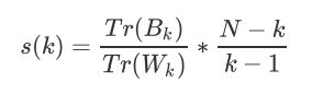
 在这里我们重点来了解一下卡林斯基-哈拉巴斯指数。Calinski-Harabaz指数越高越好。对于有k个簇的聚类而言,Calinski-Harabaz指数s(k)写作如下公式:

t2 = time()
#print(calinski_harabasz_score(x, y_pred))
t3 = time()
t_2 = t3 - t2
print(t_2) #0.0010001659393310547

import datetime
time_coumpute = datetime.datetime.fromtimestamp(t3).strftime("%Y-%m-%d %H:%M:%S")
print(time_coumpute)  #2021-11-02 13:56:18
根据对比可知,有卡林斯基-哈拉巴斯指数相比于轮廓系数来说,计算速度更快,前者计算时间是后者计算时间的五分之一。
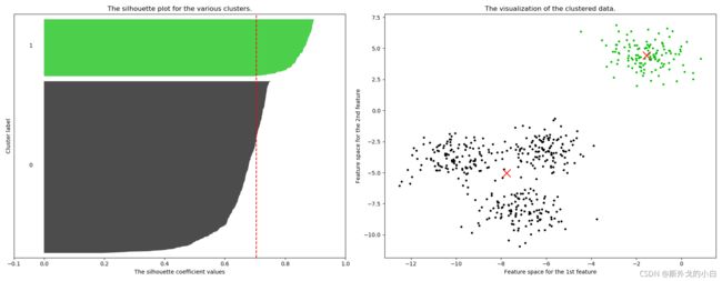
3.3案例:基于轮廓系数来选择n_clusters
from sklearn.datasets import make_blobs
from matplotlib import pyplot as plt
from sklearn.cluster import KMeans
import numpy as np
import pandas as pd
from sklearn.metrics import silhouette_samples, silhouette_score
import matplotlib.cm as cm #导入colormap

X, y = make_blobs(n_samples=500, n_features=2, centers=4, random_state=1)

for n_clusters in [2, 3, 4, 5, 6, 7]:
    n_clusters = n_clusters
    fig, (ax1, ax2) = plt.subplots(1, 2)
    fig.set_size_inches(18, 7)
    ax1.set_xlim([-0.1, 1])
    ax1.set_ylim([0, X.shape[0] + (n_clusters + 1) * 10])
    clusterer = KMeans(n_clusters=n_clusters, random_state=10).fit(X)
    cluster_labels = clusterer.labels_
    silhouette_avg = silhouette_score(X, cluster_labels)
    print("For n_clusters =", n_clusters,
          "The average silhouette_score is :", silhouette_avg)
    sample_silhouette_values = silhouette_samples(X, cluster_labels)
    y_lower = 10
    for i in range(n_clusters):
        ith_cluster_silhouette_values = sample_silhouette_values[cluster_labels == i]
        ith_cluster_silhouette_values.sort()
        size_cluster_i = ith_cluster_silhouette_values.shape[0]
        y_upper = y_lower + size_cluster_i
        color = cm.nipy_spectral(float(i) / n_clusters)
        ax1.fill_betweenx(np.arange(y_lower, y_upper)
                          , ith_cluster_silhouette_values
                          , facecolor=color
                          , alpha=0.7
                          )
        ax1.text(-0.05
                 , y_lower + 0.5 * size_cluster_i
                 , str(i))
        y_lower = y_upper + 10
    ax1.set_title("The silhouette plot for the various clusters.")
    ax1.set_xlabel("The silhouette coefficient values")
    ax1.set_ylabel("Cluster label")
    ax1.axvline(x=silhouette_avg, color="red", linestyle="--")
    ax1.set_yticks([])
    ax1.set_xticks([-0.1, 0, 0.2, 0.4, 0.6, 0.8, 1])
    colors = cm.nipy_spectral(cluster_labels.astype(float) / n_clusters)
    ax2.scatter(X[:, 0], X[:, 1]
                , marker='o'
                , s=8
                , c=colors
                )
    centers = clusterer.cluster_centers_
    # Draw white circles at cluster centers
    ax2.scatter(centers[:, 0], centers[:, 1], marker='x',
                c="red", alpha=1, s=200)

    ax2.set_title("The visualization of the clustered data.")
    ax2.set_xlabel("Feature space for the 1st feature")
    ax2.set_ylabel("Feature space for the 2nd feature")
    plt.show()
For n_clusters = 2 The average silhouette_score is : 0.7049787496083262
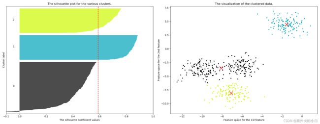
For n_clusters = 3 The average silhouette_score is : 0.5882004012129721
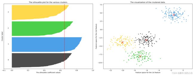 For n_clusters = 4 The average silhouette_score is : 0.6505186632729437

For n_clusters = 5 The average silhouette_score is : 0.56376469026194

For n_clusters = 6 The average silhouette_score is : 0.4504666294372765

For n_clusters = 7 The average silhouette_score is : 0.39092211029930857
3.4 重要参数init & random_state & n_init:初始质心怎么放好?
init:可输入"k-means++",“random"或者一个n维数组。这是初始化质心的方法,默认"k-means++”。输入"kmeans++":一种为K均值聚类选择初始聚类中心的聪明的办法,以加速收敛。如果输入了n维数组,数组的形状应
该是(n_clusters,n_features)并给出初始质心。
random_state:控制每次质心随机初始化的随机数种子
n_init:整数,默认10,使用不同的质心随机初始化的种子来运行k-means算法的次数。最终结果会是基于Inertia
来计算的n_init次连续运行后的最佳输出
在KMeans中,init默认使用k-means++来计算最佳质心
from sklearn.datasets import make_blobs
from matplotlib import pyplot as plt
from sklearn.cluster import KMeans
from sklearn.metrics import silhouette_score
import numpy as np
import pandas as pd
from time import time

X, y = make_blobs(n_samples=500, n_features=2, centers=4, random_state=1)

time0 = time()
plus = KMeans(n_clusters=10, random_state=0).fit(X)
time1 = time()
#print(time1 - time0) #0.09420061111450195
#print(plus.n_iter_) #迭代次数为7次

time2 = time()
random = KMeans(n_clusters=10, init="random", random_state=0).fit(X)
time3 = time()
#print(time3 - time2)  #0.04523110389709473
#print(random.n_iter_)  #迭代次数为14次
使用kmeans++寻找质心的时候,最大迭代次数较少,更快达到收敛状态。但是计算时间较长是因为在选择质心的时候浪费了一些时间。
3.5 重要参数max_iter& tol:让迭代停下来
max_iter:整数,默认300,单次运行的k-means算法的最大迭代次数
tol:浮点数,默认1e-4,两次迭代间Inertia下降的量,如果两次迭代之间Inertia下降的值小于tol所设定的值,迭代就会停下
cluster1 = KMeans(n_clusters=10, init="random", max_iter=10, random_state=420).fit(X)
y_pred_max10 = cluster1.labels_
print(silhouette_score(X, y_pred_max10)) #0.3952586444034157


cluster2 = KMeans(n_clusters=10, init="random", max_iter=20, random_state=420).fit(X)
y_pred_max20 = cluster2.labels_
print(silhouette_score(X, y_pred_max20)) #0.3401504537571701
3.6 重要属性与重要接口
from sklearn.cluster import k_means
a = k_means(X, 4, return_n_iter=True)
print(a)
#直接返回质心,inertia值,每个点的标签值、最大迭代次数
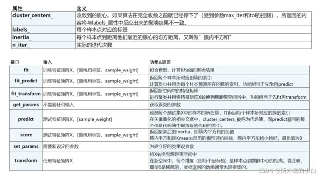
当数据量比较大的情况下,我们可以选择其中一部分来训练,此时就需要用predict对其余的数据数据哪个簇进行预测
3.7函数cluster.k_means
from sklearn.cluster import k_means
a = k_means(X, 4, return_n_iter=True)
#print(a)
#直接返回质心,inertia值,每个点的标签值、最大迭代次数
一次性地,函数k_means会依次返回质心,每个样本对应的簇的标签,inertia以及最佳迭代次数。
4、案例:聚类算法用于降维,KMeans的矢量量化应用
特征选择的降维是直接选取对模型贡献最大的特征,PCA的降维是聚合信息,而矢量量化的降维是在同等样本量上压缩信息的大小,即不改变特征的数目也不改变样本的数目,只改变在这些特征下的样本上的信息量。

import numpy as np
import pandas as pd
import matplotlib.pyplot as plt
from sklearn.cluster import KMeans
from sklearn.metrics import pairwise_distances_argmin
from sklearn.datasets import load_sample_image
from sklearn.utils import shuffle

china = load_sample_image("china.jpg")
print(china)
print(china.shape) #(427, 640, 3)
print(china[0][0]) #[174 201 231]

colors = pd.DataFrame(newimage).drop_duplicates().shape  #去重
print(colors)
(96615, 3)
#经过去重之后一共有9665种不同的像素

plt.figure(figsize=(15, 15))
plt.imshow(china)
plt.show()

flower = load_sample_image("flower.jpg")
plt.figure(figsize=(15, 15))
plt.imshow(flower)
plt.show()


n_clusters = 64
china = np.array(china, dtype=np.float64) / china.max()
w, h, d = tuple(china.shape)
#print(w, h, d)

assert d == 3 #当d维度不等于3的时候就会报错,因为图片的像素值必须是三个通道值
image_array = np.reshape(china, ((w * h), d))
#这个就等同于 china = chaina.reshape(((w * h), d))
#之所以要从三维变为二维是因为sklearn中只能对二维数据进行运算
#print(image_array.shape) #(273280, 3)

#对数据进行K-Means的矢量量化
image_array_sample = shuffle(image_array, random_state=0)[: 1000]
#随机选择1000个像素值进行训练
kmeans = KMeans(n_clusters=n_clusters, random_state=0).fit(image_array_sample)
centers = kmeans.cluster_centers_
print(centers)  #得到了每个质心的像素值

labels = kmeans.predict(image_array)
print(labels.shape)  #(273280,)#print(labels)


image_kmeans = image_array.copy()
for i in range(w * h):
    image_kmeans[i] = kmeans.cluster_centers_[labels[i]]

#print(image_kmeans)

image_kmeans = image_kmeans.reshape(w, h, d)
#print(image_kmeans.shape)  #(427, 640, 3)

#对数据进行随机的矢量化
centorid_random = shuffle(image_array, random_state=0)[:n_clusters]
#print(centorid_random)

labels_random = pairwise_distances_argmin(centorid_random, image_array, axis=0)
#挨个计算每个像素点与质心的距离,返回距离最近的质心的索引
#print(labels_random)
#[55 55 55 ... 52 60 60]

#print(labels_random.shape)  #(273280,)

image_random = image_array.copy()
for i in range(w * h):
    image_random[i] = centorid_random[labels_random[i]]

image_random = image_random.reshape(w, h, d)
print(image_random.shape) #(427, 640, 3)

fig, axes = plt.subplots(1, 3)
fig.set_size_inches(45, 15)
colors = [china, image_kmeans, image_random]
titles = ["china", "kmeans", "random"]


for i, ax in enumerate(axes.flat):
    ax.imshow(colors[i])
    ax.set_title(titles[i], fontsize=25)
    ax.set_xticks([])
    ax.set_yticks([])

plt.show()
可以看出来,kmeans进行像素聚合之后效果比随机聚合效果好,只有浅色部分由锯齿状。