图卷积 节点分类
This article goes through the implementation of Graph Convolution Networks (GCN) using Spektral API, which is a Python library for graph deep learning based on Tensorflow 2. We are going to perform Semi-Supervised Node Classification using CORA dataset, similar to the work presented in the original GCN paper by Thomas Kipf and Max Welling (2017).
本文介绍了使用 Spektral API 实现图卷积网络(GCN)的情况 ,这是一个基于Tensorflow 2的用于图深度学习的Python库。我们将使用CORA数据集执行半监督节点分类,与所介绍的工作类似在 Thomas Kipf和Max Welling(2017) 的原始GCN论文中 。
If you want to get basic understanding on Graph Convolutional Networks, it is recommended to read the first and the second parts of this series beforehand.
如果您想对图卷积网络有基本的了解,建议您 事先 阅读 本系列 的 第一 和 第二 部分。
数据集概述 (Dataset Overview)
CORA citation network dataset consists of 2708 nodes, where each node represents a document or a technical paper. The node features are bag-of-words representation that indicates the presence of a word in the document. The vocabulary — hence, also the node features — contains 1433 words.
CORA引用网络数据集由2708个节点组成,其中每个节点代表一个文档或技术论文。 节点特征是词袋表示,指示文档中单词的存在。 词汇表-因此,还有节点特征-包含1433个单词。
source 来源说明单词袋作为节点特征We will treat the dataset as an undirected graph where the edge represents whether one document cites the other or vice versa. There is no edge feature in this dataset. The goal of this task is to classify the nodes (or the documents) into 7 different classes which correspond to the papers’ research areas. This is a single-label multi-class classification problem with Single Mode data representation setting.
我们将数据集视为无向图 ,其中边表示一个文档引用了另一文档,反之亦然。 该数据集中没有边缘特征。 此任务的目标是将节点(或文档)分类为7种不同的类别,分别对应于论文的研究领域。 这是一个单标签多类别分类问题 单模式数据表示设置。
This implementation is also an example of Transductive Learning, where the neural network sees all data, including the test dataset, during the training. This is contrast to Inductive Learning — which is the typical Supervised Learning — where the test data is kept separate during the training.
此实现方式也是Transductive Learning的示例,在训练过程中,神经网络可以查看所有数据,包括测试数据集。 这与归纳学习(典型的监督学习)相反,归纳学习在训练过程中将测试数据保持独立。
文字分类问题 (Text Classification Problem)
Since we are going to classify documents based on their textual features, a common machine learning way to look at this problem is by seeing it as a supervised text classification problem. Using this approach, the machine learning model will learn each document’s hidden representation only based on its own features.
由于我们将根据文档的文本特征对文档进行分类,因此,解决此问题的一种常见的机器学习方法是将其视为有监督的文本分类问题。 使用这种方法,机器学习模型将仅基于自身的功能来学习每个文档的隐藏表示。
Illustration of text classification approach on a document classification problem (image by author) 关于文档分类问题的文本分类方法的图示(作者提供的图像)This approach might work well if there are enough labeled examples for each class. Unfortunately, in real world cases, labeling data might be expensive.
如果每个类都有足够的带标签的示例,则此方法可能会很好用。 不幸的是,在现实情况下,标记数据可能会很昂贵。
What is another approach to solve this problem?
解决此问题的另一种方法是什么?
Besides its own text content, normally, a technical paper also cites other related papers. Intuitively, the cited papers are likely to belong to similar research area.
除了自身的文本内容外,技术论文通常还会引用其他相关论文。 从直觉上讲,被引论文可能属于相似的研究领域。
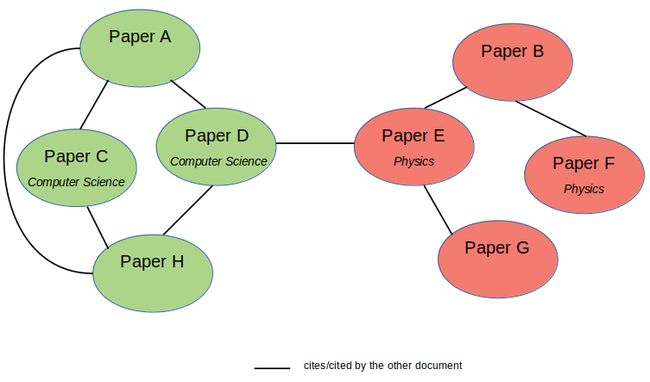
In this citation network dataset, we want to leverage the citation information from each paper in addition to its own textual content. Hence, the dataset has now turned into a network of papers.
在这个引文网络数据集中,我们希望利用每篇论文的引文信息以及自己的文本内容。 因此,数据集现在变成了论文网络。
Illustration of citation network dataset with partly labeled data (image by author) 带有部分标记数据的引文网络数据集插图(作者提供的图像)Using this configuration, we can utilize Graph Neural Networks, such as Graph Convolutional Networks (GCNs), to build a model that learns the documents interconnection in addition to their own textual features. The GCN model will learn the nodes (or documents) hidden representation not only based on its own features, but also its neighboring nodes’ features. Hence, we can reduce the number of necessary labeled examples and implement semi-supervised learning utilizing the Adjacency Matrix (A) or the nodes connectivity within a graph.
使用此配置,我们可以利用诸如图卷积网络(GCN)之类的图神经网络来构建一个模型,该模型除了学习其自身的文本特征外,还可以学习文档的互连。 GCN模型将不仅基于其自身的特征,而且还基于其邻近节点的特征,来学习节点(或文档)的隐藏表示。 因此,我们可以减少必要的带标签示例的数量,并利用邻接矩阵(A)进行半监督学习 或图中的节点连通性。
Another case where Graph Neural Networks might be useful is when each example does not have distinct features on its own, but the relations between the examples can enrich the feature representations.
图神经网络可能有用的另一种情况是,每个示例自身都不具有明显的特征,但是示例之间的关系可以丰富特征表示。
图卷积网络的实现 (Implementation of Graph Convolutional Networks)
加载和解析数据集 (Loading and Parsing the Dataset)
In this experiment, we are going to build and train a GCN model using Spektral API that is built on Tensorflow 2. Although Spektral provides built-in functions to load and preprocess CORA dataset, in this article we are going to download the raw dataset from here in order to gain deeper understanding on the data preprocessing and configuration. The complete code of the whole exercise in this article can be found on GitHub.
在此实验中,我们将使用基于Tensorflow 2构建的Spektral API来构建和训练GCN模型。尽管Spektral提供了内置功能来加载和预处理CORA数据集,但在本文中,我们将从以下位置下载原始数据集: 在这里 ,以获得对数据预处理和配置更深入的了解。 本文整个练习的完整代码可以在GitHub上找到 。
We use cora.content and cora.cites files in the respective data directory. After loading the files, we will randomly shuffle the data.
我们在各自的数据目录中使用cora.content和cora.cites文件。 加载文件后,我们将随机重新整理数据。
In cora.content file, each line consists of several elements:the first element indicates the document (or node) ID,the second until the last second elements indicate the node features,the last element indicates the label of that particular node.
在cora.content文件中,每一行包含几个元素:第一个元素指示文档(或节点)ID, 第二个直到最后一个第二元素指示节点特征, 最后一个元素指示该特定节点的标签。
In cora.cites file, each line contains a tuple of documents (or nodes) IDs. The first element of the tuple indicates the ID of the paper being cited, while the second element indicates the paper containing the citation. Although this configuration represents a directed graph, in this approach we treat the dataset as an undirected graph.
在cora.cites文件中,每行包含一个文档(或节点)ID的元组。 元组的第一个元素指示被引用论文的ID ,而第二个元素指示包含被引用论文 。 尽管此配置表示有向图,但是在这种方法中,我们将数据集视为无向图 。
After loading the data, we build Node Features Matrix (X) and a list containing tuples of adjacent nodes. This edges list will be used to build a graph from where we can obtain the Adjacency Matrix (A).
加载数据后,我们构建节点特征矩阵( X )和一个包含相邻节点元组的列表。 此边缘列表将用于构建图,从中可以获取邻接矩阵( A )。
Output:
输出:
设置训练,验证和测试掩码 (Setting the Train, Validation, and Test Mask)
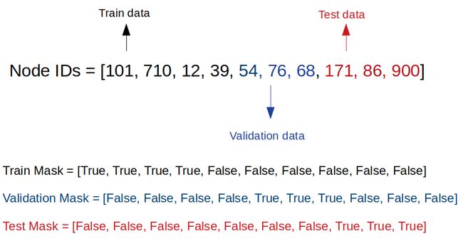
We will feed in the Node Features Matrix (X) and Adjacency Matrix (A) to the neural networks. We are also going to set Boolean masks with a length of N for each training, validation, and testing dataset. The elements of those masks are True when they belong to corresponding training, validation, or test dataset. For example, the elements of train mask are True for those which belong to training data.
我们将节点特征矩阵( X )和邻接矩阵( A )馈入神经网络。 我们还将为每个设置长度为N的 布尔掩码 训练,验证和测试数据集。 这些遮罩的元素属于相应的训练,验证或测试数据集时,它们为True 。 例如,对于属于训练数据的那些元素,训练蒙版的元素为True 。
Examples of Train, Validation, and Test Boolean Masks 训练,验证和测试布尔掩码的示例In the paper, they pick 20 labeled examples for each class. Hence, with 7 classes, we will have a total of 140 labeled training examples. We will also use 500 labeled validation examples and 1000 labeled testing examples.
在本文中,他们为每个班级选取20个带有标签的示例。 因此,通过7个课程,我们将总共有140个带有标签的培训示例。 我们还将使用500个带标签的验证示例和1000个带标签的测试示例。
获取邻接矩阵 (Obtaining the Adjacency Matrix)
The next step is to obtain the Adjacency Matrix (A) of the graph. We use NetworkX to help us do this. We will initialize a graph and then add the nodes and edges lists to the graph.
下一步是获取图的邻接矩阵( A )。 我们使用NetworkX来帮助我们做到这一点。 我们将初始化一个图,然后将节点和边列表添加到图中。
Output:
输出:
将标签转换为一键编码 (Converting the label to one-hot encoding)
The last step before building our GCN is, just like any other machine learning model, encoding the labels and then converting them to one-hot encoding.
与其他任何机器学习模型一样,构建GCN之前的最后一步是对标签进行编码,然后将其转换为一次性编码。
We are now done with data preprocessing and ready to build our GCN!
现在,我们已经完成了数据预处理,并准备构建我们的GCN!
建立图卷积网络 (Build the Graph Convolutional Networks)
The GCN model architectures and hyperparameters follow the design from GCN original paper. The GCN model will take 2 inputs, the Node Features Matrix (X) and Adjacency Matrix (A). We are going to implement 2-layer GCN with Dropout layers and L2 regularization. We are also going to set the maximum training epochs to be 200 and implement Early Stopping with patience of 10. It means that the training will be stopped once the validation loss does not decrease for 10 consecutive epochs. To monitor the training and validation accuracy and loss, we are also going to call TensorBoard in the callbacks.
GCN模型的体系结构和超参数遵循GCN原始论文的设计。 GCN模型将采用2个输入,即节点特征矩阵( X )和邻接矩阵( A )。 我们将使用 Dropout层和 L2正则化实现2层GCN 。 我们还将最大训练时间设为200,并以10的耐心实施“ 提前停止” 。 这意味着一旦验证损失连续10个周期没有减少,训练就会停止。 为了监控训练和验证的准确性和损失,我们还将在回调中调用TensorBoard 。
Before feeding in the Adjacency Matrix (A) to the GCN, we need to do extra preprocessing by performing renormalization trick according to the original paper. You can also read about how renormalization trick affects GCN forward propagation calculation here.
在将邻接矩阵( A )输入到GCN之前,我们需要根据原始论文通过执行重新规范化技巧来进行额外的预处理。 您还可以阅读有关重归一化技巧如何影响GCN前向传播计算的信息 在这里 。
The code to train GCN below was originally obtained from Spektral GitHub page.
下面训练GCN的代码最初是从Spektral GitHub页面获得的。
训练图卷积网络 (Train the Graph Convolutional Networks)
We are implementing Transductive Learning, which means we will feed the whole graph to both training and testing. We separate the training, validation, and testing data using the Boolean masks we have constructed before. These masks will be passed to sample_weight argument. We set the batch_size to be the whole graph size, otherwise the graph will be shuffled.
我们正在实施“归纳式学习”,这意味着我们将把整个图表馈送给培训和测试。 我们使用之前构造的布尔掩码将训练,验证和测试数据分开。 这些掩码将传递给sample_weight参数。 我们将batch_size设置为整个图的大小,否则该图将被重新排序。
To better evaluate the model performance for each class, we use F1-score instead of accuracy and loss metrics.
为了更好地评估每个类别的模型性能,我们使用F1评分而不是准确性和损失指标。
Training done!
培训完成!
From the classification report, we obtain macro average F1-score of 74%.
从分类报告中,我们获得74%的宏观平均F1得分。
使用t-SNE的隐藏层激活可视化 (Hidden Layers Activation Visualization using t-SNE)
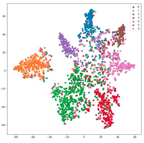
Let’s now use t-SNE to visualize the hidden layer representations. We use t-SNE to reduce the dimension of the hidden representations to 2-D. Each point in the plot represents each node (or document), while each color represents each class.
现在让我们使用t-SNE可视化隐藏层表示。 我们使用t-SNE将隐藏表示的尺寸减小为2D。 图中的每个点代表每个节点(或文档),而每种颜色代表每个类别。
Output:
输出:
T-SNE Representation of GCN Hidden Layer. GCN is able to learn features representations considerably well, shown by distinct data clusters. GCN隐藏层的T-SNE表示。 GCN能够很好地学习特征表示,由不同的数据集群显示。与完全连接的神经网络的比较 (Comparison to Fully Connected Neural Networks)
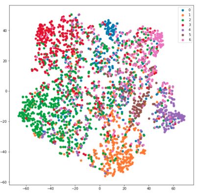
As a benchmark, I also trained a 2-layer Fully Connected Neural Networks (FCNN) and plot the t-SNE visualization of hidden layer representations. The results are shown below:
作为基准,我还训练了2层全连接神经网络(FCNN),并绘制了隐藏层表示的t-SNE可视化。 结果如下所示:
Classification Results from 2-layer Fully Connected Neural Networks 2层全连接神经网络的分类结果 T-SNE Representation of FCNN Hidden Layer Representation. FCNN cannot classify the documents as well as GCN. FCNN隐藏层表示的T-SNE表示。 FCNN无法对文档以及GCN进行分类。From the results above, it is clear that GCN significantly outperforms FCNN with macro average F1-score is only 55%. The t-SNE visualization plot of FCNN hidden layer representations is scattered, which means that FCNN can’t learn the features representations as well as GCN.
从以上结果可以明显看出,GCN的性能明显优于FCNN,宏观平均F1得分仅为55%。 FCNN隐藏层表示的t-SNE可视化图是分散的,这意味着FCNN无法像GCN一样学习特征表示。
结论 (Conclusion)
The conventional machine learning approach to perform document classification, for example CORA dataset, is to use supervised text classification approach. Graph Convolutional Networks (GCNs) is an alternative semi-supervised approach to solve this problem by seeing the documents as a network of related papers. Using only 20 labeled examples for each class, GCNs outperform Fully-Connected Neural Networks on this task by around 20%.
执行文档分类的常规机器学习方法(例如CORA数据集)是使用监督文本分类方法。 图卷积网络(GCN)是通过将文档视为相关论文的网络来解决此问题的另一种半监督方法。 对于每个类别,仅使用20个带有标签的示例,GCN在此任务上的性能就比全连接神经网络高出约20%。
Thanks for reading! I hope this article helps you implement Graph Convolutional Networks (GCNs) on your own problems.
谢谢阅读! 我希望本文能帮助您针对自己的问题实现图卷积网络(GCN)。
Any comment, feedback, or want to discuss? Just drop me a message. You can reach me on LinkedIn.
有任何意见,反馈或要讨论吗? 请给我留言。 您可以在 LinkedIn上与 我联系 。
You can find the full code on GitHub.
您可以在 GitHub上 找到完整的代码 。
翻译自: https://towardsdatascience.com/graph-convolutional-networks-on-node-classification-2b6bbec1d042
图卷积 节点分类


