OpenCV之core 模块. 核心功能(2)基本绘图 随机数发生器&绘制文字 离散傅立叶变换 输入输出XML和YAML文件 与 OpenCV 1 同时使用

基本绘图

目的

本节你将学到:

  • 如何用 Point 在图像中定义 2D 点
  • 如何以及为何使用 Scalar
  • 用OpenCV的函数 line 绘 直线
  • 用OpenCV的函数 ellipse 绘 椭圆
  • 用OpenCV的函数 rectangle 绘 矩形
  • 用OpenCV的函数 circle 绘 
  • 用OpenCV的函数 fillPoly 绘 填充的多边形

OpenCV 原理

本节中,我门将大量使用 Point 和 Scalar 这两个结构:

Point

次数据结构表示了由其图像坐标  x 和  y 指定的2D点。可定义为:
Point pt;
pt.x = 10;
pt.y = 8;

或者

Point pt =  Point(10, 8);

Scalar

  • 表示了具有4个元素的数组。次类型在OpenCV中被大量用于传递像素值。

  • 本节中,我们将进一步用它来表示RGB颜色值(三个参数)。如果用不到第四个参数,则无需定义。

  • 我们来看个例子,如果给出以下颜色参数表达式:

    Scalar( a, b, c )
    

    那么定义的RGB颜色值为: Red = cGreen = b and Blue = a

代码

  • 这些代码都来自OpenCV代码的sample文件夹。或者可 点击此处 获取。

代码分析

  1. 我们打算画两个例子(原子和赌棍), 所以必须创建两个图像和对应的窗口以显示。

    /// 窗口名字
    char atom_window[] = "Drawing 1: Atom";
    char rook_window[] = "Drawing 2: Rook";
    
    /// 创建空全黑像素的空图像
    Mat atom_image = Mat::zeros( w, w, CV_8UC3 );
    Mat rook_image = Mat::zeros( w, w, CV_8UC3 );
    
  2. 创建用来画不同几何形状的函数。比如用 MyEllipse 和 MyFilledCircle 来画原子。

    /// 1. 画一个简单的原子。
    
    /// 1.a. 创建椭圆
    MyEllipse( atom_image, 90 );
    MyEllipse( atom_image, 0 );
    MyEllipse( atom_image, 45 );
    MyEllipse( atom_image, -45 );
    
    /// 1.b. 创建圆
    MyFilledCircle( atom_image, Point( w/2.0, w/2.0) );
    
  3. 接下来用 MyLine*,*rectangle 和 a MyPolygon 来画赌棍:

    /// 2. 画一个赌棍
    
    /// 2.a. 创建一个凸多边形
    MyPolygon( rook_image );
    
    /// 2.b. 创建矩形
    rectangle( rook_image,
               Point( 0, 7*w/8.0 ),
               Point( w, w),
               Scalar( 0, 255, 255 ),
               -1,
               8 );
    
    /// 2.c. 画几条直线
    MyLine( rook_image, Point( 0, 15*w/16 ), Point( w, 15*w/16 ) );
    MyLine( rook_image, Point( w/4, 7*w/8 ), Point( w/4, w ) );
    MyLine( rook_image, Point( w/2, 7*w/8 ), Point( w/2, w ) );
    MyLine( rook_image, Point( 3*w/4, 7*w/8 ), Point( 3*w/4, w ) );
    
  4. 现在来看看每个函数内部如何定义:

    • MyLine

      void MyLine( Mat img, Point start, Point end )
      {
        int thickness = 2;
        int lineType = 8;
        line( img,
              start,
              end,
              Scalar( 0, 0, 0 ),
              thickness,
              lineType );
      }
      

      正如我们所见, MyLine 调用函数 line 来实现以下操作:

      • 画一条从点 start 到点 end 的直线段
      • 此线段将被画到图像 img 上
      • 线的颜色由 Scalar( 0, 0, 0) 来定义,在此其相应RGB值为 黑色
      • 线的粗细由 thickness 设定(此处设为 2)
      • 此线为8联通 (lineType = 8)
    • MyEllipse

      void MyEllipse( Mat img, double angle )
      {
        int thickness = 2;
        int lineType = 8;
      
        ellipse( img,
                 Point( w/2.0, w/2.0 ),
                 Size( w/4.0, w/16.0 ),
                 angle,
                 0,
                 360,
                 Scalar( 255, 0, 0 ),
                 thickness,
                 lineType );
      }
      

      根据以上代码,我们可看到函数 ellipse 按照以下规则绘制椭圆:

      • 椭圆将被画到图像 img 上
      • 椭圆中心为点 (w/2.0, w/2.0) 并且大小位于矩形 (w/4.0, w/16.0) 内
      • 椭圆旋转角度为 angle
      • 椭圆扩展的弧度从 0 度到 360 度
      • 图形颜色为 Scalar( 255, 255, 0) ,既蓝色
      • 绘椭圆的线粗为 thickness ,此处是2
    • MyFilledCircle

      void MyFilledCircle( Mat img, Point center )
      {
       int thickness = -1;
       int lineType = 8;
      
       circle( img,
               center,
               w/32.0,
               Scalar( 0, 0, 255 ),
               thickness,
               lineType );
      }
      

      类似于椭圆函数,我们可以看到 circle 函数的参数意义如下:

      • 圆将被画到图像 ( img )上
      • 圆心由点 center 定义
      • 圆的半径为: w/32.0
      • 圆的颜色为: Scalar(0, 0, 255) ,按BGR的格式为 红色
      • 线粗定义为 thickness = -1, 因此次圆将被填充
    • MyPolygon

      void MyPolygon( Mat img )
      {
        int lineType = 8;
      
        /** 创建一些点 */
        Point rook_points[1][20];
        rook_points[0][0] = Point( w/4.0, 7*w/8.0 );
        rook_points[0][1] = Point( 3*w/4.0, 7*w/8.0 );
        rook_points[0][2] = Point( 3*w/4.0, 13*w/16.0 );
        rook_points[0][3] = Point( 11*w/16.0, 13*w/16.0 );
        rook_points[0][4] = Point( 19*w/32.0, 3*w/8.0 );
        rook_points[0][5] = Point( 3*w/4.0, 3*w/8.0 );
        rook_points[0][6] = Point( 3*w/4.0, w/8.0 );
        rook_points[0][7] = Point( 26*w/40.0, w/8.0 );
        rook_points[0][8] = Point( 26*w/40.0, w/4.0 );
        rook_points[0][9] = Point( 22*w/40.0, w/4.0 );
        rook_points[0][10] = Point( 22*w/40.0, w/8.0 );
        rook_points[0][11] = Point( 18*w/40.0, w/8.0 );
        rook_points[0][12] = Point( 18*w/40.0, w/4.0 );
        rook_points[0][13] = Point( 14*w/40.0, w/4.0 );
        rook_points[0][14] = Point( 14*w/40.0, w/8.0 );
        rook_points[0][15] = Point( w/4.0, w/8.0 );
        rook_points[0][16] = Point( w/4.0, 3*w/8.0 );
        rook_points[0][17] = Point( 13*w/32.0, 3*w/8.0 );
        rook_points[0][18] = Point( 5*w/16.0, 13*w/16.0 );
        rook_points[0][19] = Point( w/4.0, 13*w/16.0) ;
      
        const Point* ppt[1] = { rook_points[0] };
        int npt[] = { 20 };
      
        fillPoly( img,
                  ppt,
                  npt,
                  1,
                  Scalar( 255, 255, 255 ),
                  lineType );
       }
      
      
       我们用函数 :fill_poly:`fillPoly <>` 来绘制填充的多边形。请注意:
      • 多边形将被画到图像 img 上
      • 多边形的顶点集为 ppt
      • 要绘制的多边形顶点数目为 npt
      • 要绘制的多边形数量仅为 1
      • 多边形的颜色定义为 Scalar( 255, 255, 255), 既BGR值为 白色
    • rectangle

      rectangle( rook_image,
                 Point( 0, 7*w/8.0 ),
                 Point( w, w),
                 Scalar( 0, 255, 255 ),
                 -1,
                 8 );
      

      最后是函数:rectangle:rectangle <> (我们并没有为这家伙创建特定函数)。请注意:

      • 矩形将被画到图像 rook_image 上
      • 矩形两个对角顶点为 Point( 0, 7*w/8.0 ) 和 Point( w, w)
      • 矩形的颜色为 Scalar(0, 255, 255) ,既BGR格式下的 黄色
      • 由于线粗为 -1, 此矩形将被填充

结果

编译并运行例程,你将看到如下结果:

OpenCV之core 模块. 核心功能(2)基本绘图 随机数发生器&绘制文字 离散傅立叶变换 输入输出XML和YAML文件 与 OpenCV 1 同时使用_第1张图片


随机数发生器&绘制文字

目的

本节你将学到:

  • 使用 随机数发生器类 (RNG) 并得到均匀分布的随机数。
  • 通过使用函数 putText 显示文字。

代码

  • 在之前的章节中 (基本绘图) 我们绘制过不同的几何图形, 我提供了一些绘制参数,比如 coordinates(坐标) (在绘制点Points 的时候 ), color(颜色), thickness(线条-粗细,点-大小), 等等... ,你会发现我们给出了这些参数明确的数值。
  • 在本章中, 我们会试着赋予这些参数 random随机 的数值。 并且, 我们会试图在图像上绘制大量的几何图形. 因为我们将用随机的方式初始化这些图形, 这个过程将很自然的用到 loops循环 .
  • 本代码在OpenCV的sample文件夹下,如果招不到,你可以从这里 here 得到它: .

说明

  1. 让我们检视 main 函数。我们发现第一步是实例化一个 Random Number Generator(随机数发生器对象) (RNG):

    RNG rng( 0xFFFFFFFF );
    

    RNG的实现了一个随机数发生器。 在上面的例子中, rng 是用数值 0xFFFFFFFF 来实例化的一个RNG对象。

  2. 然后我们初始化一个 0 矩阵(代表一个全黑的图像), 并且指定它的宽度,高度,和像素格式:

    /// 初始化一个0矩阵
    Mat image = Mat::zeros( window_height, window_width, CV_8UC3 );
    
    /// 把它会知道一个窗口中
    imshow( window_name, image );
    
  3. 然后我们开始疯狂的绘制。看过代码时候你会发现它主要分八个部分,正如函数定义的一样:

    /// 现在我们先画线
    c = Drawing_Random_Lines(image, window_name, rng);
    if( c != 0 ) return 0;
    
    /// 继续,这次是一些矩形
    c = Drawing_Random_Rectangles(image, window_name, rng);
    if( c != 0 ) return 0;
    
    /// 画一些弧线
    c = Drawing_Random_Ellipses( image, window_name, rng );
    if( c != 0 ) return 0;
    
    /// 画一些折线
    c = Drawing_Random_Polylines( image, window_name, rng );
    if( c != 0 ) return 0;
    
    /// 画被填充的多边形
    c = Drawing_Random_Filled_Polygons( image, window_name, rng );
    if( c != 0 ) return 0;
    
    /// 画圆
    c = Drawing_Random_Circles( image, window_name, rng );
    if( c != 0 ) return 0;
    
    /// 在随机的地方绘制文字
    c = Displaying_Random_Text( image, window_name, rng );
    if( c != 0 ) return 0;
    
    /// Displaying the big end!
    c = Displaying_Big_End( image, window_name, rng );
    

    所有这些范数都遵循相同的模式,所以我们只分析其中的一组,因为这适用于所有。

  4. 查看函数 Drawing_Random_Lines:

    int Drawing_Random_Lines( Mat image, char* window_name, RNG rng )
    {
      int lineType = 8;
      Point pt1, pt2;
    
      for( int i = 0; i < NUMBER; i++ )
      {
       pt1.x = rng.uniform( x_1, x_2 );
       pt1.y = rng.uniform( y_1, y_2 );
       pt2.x = rng.uniform( x_1, x_2 );
       pt2.y = rng.uniform( y_1, y_2 );
    
       line( image, pt1, pt2, randomColor(rng), rng.uniform(1, 10), 8 );
       imshow( window_name, image );
       if( waitKey( DELAY ) >= 0 )
       { return -1; }
      }
      return 0;
    }
    

    我们可以看到:

    • for 循环将重复 NUMBER 次。 并且函数 line 在循环中, 这意味着要生成 NUMBER 条线段。

    • 线段的两个端点分别是 pt1 和 pt2. 对于 pt1 我们看到:

      pt1.x = rng.uniform( x_1, x_2 );
      pt1.y = rng.uniform( y_1, y_2 );
      
      • 我们知道 rng 是一个 随机数生成器 对象。在上面的代码中我们调用了 rng.uniform(a,b) 。这指定了一个在 a和 b 之间的均匀分布(包含 a, 但不含 b)。

      • 由上面的说明,我们可以推断出 pt1 和 pt2 将会是随机的数值,因此产生的线段是变幻不定的,这会产生一个很好的视觉效果(从下面绘制的图片可以看出)。

      • 我们还可以发现, 在 line 的参数设置中,对于 color 的设置我们用了:

        randomColor(rng)
        

        让我们来看看函数的实现:

        static Scalar randomColor( RNG& rng )
          {
          int icolor = (unsigned) rng;
          return Scalar( icolor&255, (icolor>>8)&255, (icolor>>16)&255 );
          }
        

        正如我们看到的,函数的返回值是一个用三个随机数初始化的 Scalar 对象,这三个随机数代表了颜色的 RGB分量。所以,线段的颜色也是随机的!

  5. 上面的解释同样适用于其它的几何图形,比如说参数 center(圆心) 和 vertices(顶点) 也是随机的。

  6. 在结束之前,我们还应该看看函数 Display_Random_Text 和 Displaying_Big_End, 因为它们有一些有趣的特征:

  7. Display_Random_Text:

    int Displaying_Random_Text( Mat image, char* window_name, RNG rng )
    {
      int lineType = 8;
    
      for ( int i = 1; i < NUMBER; i++ )
      {
        Point org;
        org.x = rng.uniform(x_1, x_2);
        org.y = rng.uniform(y_1, y_2);
    
        putText( image, "Testing text rendering", org, rng.uniform(0,8),
                 rng.uniform(0,100)*0.05+0.1, randomColor(rng), rng.uniform(1, 10), lineType);
    
        imshow( window_name, image );
        if( waitKey(DELAY) >= 0 )
          { return -1; }
      }
    
      return 0;
    }
    

    这些看起来都很熟悉,但是这一句:

    putText( image, "Testing text rendering", org, rng.uniform(0,8),
             rng.uniform(0,100)*0.05+0.1, randomColor(rng), rng.uniform(1, 10), lineType);
    

    函数 putText 都做了些什么?在我们的例子中:

    • 在 image 上绘制文字 “Testing text rendering” 。
    • 文字的左下角将用点 org 指定。
    • 字体参数是用一个在 [0, 8> 之间的整数来定义。
    • 字体的缩放比例是用表达式 rng.uniform(0, 100)x0.05 + 0.1 指定(表示它的范围是 [0.1, 5.1>)。
    • 字体的颜色是随机的 (记为 randomColor(rng))。
    • 字体的粗细范围是从 1 到 10, 表示为 rng.uniform(1,10) 。

    因此, 我们将绘制 (与其余函数类似) NUMBER 个文字到我们的图片上,以位置随机的方式。

  8. Displaying_Big_End

    int Displaying_Big_End( Mat image, char* window_name, RNG rng )
    {
      Size textsize = getTextSize("OpenCV forever!", CV_FONT_HERSHEY_COMPLEX, 3, 5, 0);
      Point org((window_width - textsize.width)/2, (window_height - textsize.height)/2);
      int lineType = 8;
    
      Mat image2;
    
      for( int i = 0; i < 255; i += 2 )
      {
        image2 = image - Scalar::all(i);
        putText( image2, "OpenCV forever!", org, CV_FONT_HERSHEY_COMPLEX, 3,
               Scalar(i, i, 255), 5, lineType );
    
        imshow( window_name, image2 );
        if( waitKey(DELAY) >= 0 )
          { return -1; }
      }
    
      return 0;
    }
    

    除了 getTextSize (用于获取文字的大小参数), 我们可以发现在 for 循环里的新操作:

      image2 = image - Scalar::all(i)
    
    **image2** 是 **image** 和 **Scalar::all(i)** 的差。事实上,**image2** 的每个像素都是 **image** 的每个像素减去 **i** (对于每个像素,都是由R,G,B三个分量组成,每个分量都会独立做差)的差。
我们还要知道,减法操作  总是 保证是  合理 的操作, 这表明结果总是在合理的范围内 (这个例子里结果不会为负数,并且保证在 0~255的合理范围内)。

结果

正如你在代码部分看到的, 程序将依次执行不同的绘图函数,这将:

  1. 首先 NUMBER 条线段将出现在屏幕上,正如截图所示:
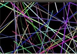
    OpenCV之core 模块. 核心功能(2)基本绘图 随机数发生器&绘制文字 离散傅立叶变换 输入输出XML和YAML文件 与 OpenCV 1 同时使用_第2张图片
  2. 然后,一个新的图形,这次是一些矩形:

  3. 现在,一些弧线会出现,每一个弧线都有随机的位置,大小,边缘的粗细和弧长:

    OpenCV之core 模块. 核心功能(2)基本绘图 随机数发生器&绘制文字 离散傅立叶变换 输入输出XML和YAML文件 与 OpenCV 1 同时使用_第3张图片
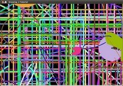
  4. 现在,带有三个参数的 polylines(折线) 将会出现在屏幕上,同样以随机的方式:

    OpenCV之core 模块. 核心功能(2)基本绘图 随机数发生器&绘制文字 离散傅立叶变换 输入输出XML和YAML文件 与 OpenCV 1 同时使用_第4张图片
  5. 填充的多边形 (这里是三角形) 会出现.

  6. 最后出现的图形:圆

    OpenCV之core 模块. 核心功能(2)基本绘图 随机数发生器&绘制文字 离散傅立叶变换 输入输出XML和YAML文件 与 OpenCV 1 同时使用_第5张图片
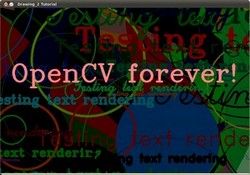
  7. 在结尾处,文字 “Testing Text Rendering” 将会以不同的字体,大小,颜色和位置出现在屏幕上。

  8. 最后 (这也顺便表达了OpenCV的宗旨):

    OpenCV之core 模块. 核心功能(2)基本绘图 随机数发生器&绘制文字 离散傅立叶变换 输入输出XML和YAML文件 与 OpenCV 1 同时使用_第6张图片


离散傅立叶变换

目标

本文档尝试解答如下问题:

  • 什么是傅立叶变换及其应用?
  • 如何使用OpenCV提供的傅立叶变换?
  • 相关函数的使用,如: copyMakeBorder(), merge(), dft(), getOptimalDFTSize(), log() 和 normalize() .

源码

你可以 从此处下载源码 或者通过OpenCV源码库文件samples/cpp/tutorial_code/core/discrete_fourier_transform/discrete_fourier_transform.cpp 查看.

以下为函数 dft() 使用范例:

 1
 2
 3
 4
 5
 6
 7
 8
 9
10
11
12
13
14
15
16
17
18
19
20
21
22
23
24
25
26
27
28
29
30
31
32
33
34
35
36
37
38
39
40
41
42
43
44
45
46
47
48
49
50
51
52
53
54
55
56
57
58
59
60
61
62
#include "opencv2/core/core.hpp"
#include "opencv2/imgproc/imgproc.hpp"
#include "opencv2/highgui/highgui.hpp"
#include 
int main(int argc, char ** argv)
{
    const char* filename = argc >=2 ? argv[1] : "lena.jpg";

    Mat I = imread(filename, CV_LOAD_IMAGE_GRAYSCALE);
    if( I.empty())
        return -1;
    
    Mat padded;                            //expand input image to optimal size
    int m = getOptimalDFTSize( I.rows );
    int n = getOptimalDFTSize( I.cols ); // on the border add zero values
    copyMakeBorder(I, padded, 0, m - I.rows, 0, n - I.cols, BORDER_CONSTANT, Scalar::all(0));

    Mat planes[] = {Mat_<float>(padded), Mat::zeros(padded.size(), CV_32F)};
    Mat complexI;
    merge(planes, 2, complexI);         // Add to the expanded another plane with zeros

    dft(complexI, complexI);            // this way the result may fit in the source matrix

    // compute the magnitude and switch to logarithmic scale
    // => log(1 + sqrt(Re(DFT(I))^2 + Im(DFT(I))^2))
    split(complexI, planes);                   // planes[0] = Re(DFT(I), planes[1] = Im(DFT(I))
    magnitude(planes[0], planes[1], planes[0]);// planes[0] = magnitude  
    Mat magI = planes[0];
    
    magI += Scalar::all(1);                    // switch to logarithmic scale
    log(magI, magI);

    // crop the spectrum, if it has an odd number of rows or columns
    magI = magI(Rect(0, 0, magI.cols & -2, magI.rows & -2));

    // rearrange the quadrants of Fourier image  so that the origin is at the image center        
    int cx = magI.cols/2;
    int cy = magI.rows/2;

    Mat q0(magI, Rect(0, 0, cx, cy));   // Top-Left - Create a ROI per quadrant 
    Mat q1(magI, Rect(cx, 0, cx, cy));  // Top-Right
    Mat q2(magI, Rect(0, cy, cx, cy));  // Bottom-Left
    Mat q3(magI, Rect(cx, cy, cx, cy)); // Bottom-Right

    Mat tmp;                           // swap quadrants (Top-Left with Bottom-Right)
    q0.copyTo(tmp);
    q3.copyTo(q0);
    tmp.copyTo(q3);

    q1.copyTo(tmp);                    // swap quadrant (Top-Right with Bottom-Left)
    q2.copyTo(q1);
    tmp.copyTo(q2);

    normalize(magI, magI, 0, 1, CV_MINMAX); // Transform the matrix with float values into a 
                                            // viewable image form (float between values 0 and 1).

    imshow("Input Image"       , I   );    // Show the result
    imshow("spectrum magnitude", magI);    
    waitKey();

    return 0;
}

原理

对一张图像使用傅立叶变换就是将它分解成正弦和余弦两部分。也就是将图像从空间域(spatial domain)转换到频域(frequency domain)。 这一转换的理论基础来自于以下事实:任一函数都可以表示成无数个正弦和余弦函数的和的形式。傅立叶变换就是一个用来将函数分解的工具。 2维图像的傅立叶变换可以用以下数学公式表达:

F(k,l) = \displaystyle\sum\limits_{i=0}^{N-1}\sum\limits_{j=0}^{N-1} f(i,j)e^{-i2\pi(\frac{ki}{N}+\frac{lj}{N})}e^{ix} = \cos{x} + i\sin {x}

式中 f 是空间域(spatial domain)值, F 则是频域(frequency domain)值。 转换之后的频域值是复数, 因此,显示傅立叶变换之后的结果需要使用实数图像(real image) 加虚数图像(complex image), 或者幅度图像(magitude image)加相位图像(phase image)。 在实际的图像处理过程中,仅仅使用了幅度图像,因为幅度图像包含了原图像的几乎所有我们需要的几何信息。 然而,如果你想通过修改幅度图像或者相位图像的方法来间接修改原空间图像,你需要使用逆傅立叶变换得到修改后的空间图像,这样你就必须同时保留幅度图像和相位图像了。

在此示例中,我将展示如何计算以及显示傅立叶变换后的幅度图像。由于数字图像的离散性,像素值的取值范围也是有限的。比如在一张灰度图像中,像素灰度值一般在0到255之间。 因此,我们这里讨论的也仅仅是离散傅立叶变换(DFT)。 如果你需要得到图像中的几何结构信息,那你就要用到它了。请参考以下步骤(假设输入图像为单通道的灰度图像 I):

  1. 将图像延扩到最佳尺寸. 离散傅立叶变换的运行速度与图片的尺寸息息相关。当图像的尺寸是2, 3,5的整数倍时,计算速度最快。 因此,为了达到快速计算的目的,经常通过添凑新的边缘像素的方法获取最佳图像尺寸。函数 getOptimalDFTSize()返回最佳尺寸,而函数 copyMakeBorder() 填充边缘像素:

    Mat padded;                            //将输入图像延扩到最佳的尺寸
    int m = getOptimalDFTSize( I.rows );
    int n = getOptimalDFTSize( I.cols ); // 在边缘添加0
    copyMakeBorder(I, padded, 0, m - I.rows, 0, n - I.cols, BORDER_CONSTANT, Scalar::all(0));
    

    添加的像素初始化为0.

  2. 为傅立叶变换的结果(实部和虚部)分配存储空间. 傅立叶变换的结果是复数,这就是说对于每个原图像值,结果是两个图像值。 此外,频域值范围远远超过空间值范围, 因此至少要将频域储存在 float 格式中。 结果我们将输入图像转换成浮点类型,并多加一个额外通道来储存复数部分:

    Mat planes[] = {Mat_<float>(padded), Mat::zeros(padded.size(), CV_32F)};
    Mat complexI;
    merge(planes, 2, complexI);         // 为延扩后的图像增添一个初始化为0的通道
    
  3. 进行离散傅立叶变换. 支持图像原地计算 (输入输出为同一图像):

    dft(complexI, complexI);            // 变换结果很好的保存在原始矩阵中
    
  4. 将复数转换为幅度.复数包含实数部分(Re)和复数部分 (imaginary - Im)。 离散傅立叶变换的结果是复数,对应的幅度可以表示为:

    M = \sqrt[2]{ {Re(DFT(I))}^2 + {Im(DFT(I))}^2}

转化为OpenCV代码:

split(complexI, planes);                   // planes[0] = Re(DFT(I), planes[1] = Im(DFT(I))
magnitude(planes[0], planes[1], planes[0]);// planes[0] = magnitude
Mat magI = planes[0];
  1. 对数尺度(logarithmic scale)缩放. 傅立叶变换的幅度值范围大到不适合在屏幕上显示。高值在屏幕上显示为白点,而低值为黑点,高低值的变化无法有效分辨。为了在屏幕上凸显出高低变化的连续性,我们可以用对数尺度来替换线性尺度:

    M_1 = \log{(1 + M)}

    转化为OpenCV代码:

    magI += Scalar::all(1);                    // 转换到对数尺度
    log(magI, magI);
    
  2. 剪切和重分布幅度图象限. 还记得我们在第一步时延扩了图像吗? 那现在是时候将新添加的像素剔除了。为了方便显示,我们也可以重新分布幅度图象限位置(注:将第五步得到的幅度图从中间划开得到四张1/4子图像,将每张子图像看成幅度图的一个象限,重新分布即将四个角点重叠到图片中心)。 这样的话原点(0,0)就位移到图像中心。

    magI = magI(Rect(0, 0, magI.cols & -2, magI.rows & -2));
    int cx = magI.cols/2;
    int cy = magI.rows/2;
    
    Mat q0(magI, Rect(0, 0, cx, cy));   // Top-Left - 为每一个象限创建ROI
    Mat q1(magI, Rect(cx, 0, cx, cy));  // Top-Right
    Mat q2(magI, Rect(0, cy, cx, cy));  // Bottom-Left
    Mat q3(magI, Rect(cx, cy, cx, cy)); // Bottom-Right
    
    Mat tmp;                           // 交换象限 (Top-Left with Bottom-Right)
    q0.copyTo(tmp);
    q3.copyTo(q0);
    tmp.copyTo(q3);
    
    q1.copyTo(tmp);                    // 交换象限 (Top-Right with Bottom-Left)
    q2.copyTo(q1);
    tmp.copyTo(q2);
    
  3. 归一化. 这一步的目的仍然是为了显示。 现在我们有了重分布后的幅度图,但是幅度值仍然超过可显示范围[0,1] 。我们使用normalize() 函数将幅度归一化到可显示范围。

normalize(magI, magI, 0, 1, CV_MINMAX); // 将float类型的矩阵转换到可显示图像范围
                                        // (float [0, 1]).

结果

离散傅立叶变换的一个应用是决定图片中物体的几何方向.比如,在文字识别中首先要搞清楚文字是不是水平排列的? 看一些文字,你就会注意到文本行一般是水平的而字母则有些垂直分布。文本段的这两个主要方向也是可以从傅立叶变换之后的图像看出来。我们使用这个 水平文本图像 以及 旋转文本图像 来展示离散傅立叶变换的结果 。

水平文本图像:

In case of normal text

旋转文本图像:

In case of rotated text

观察这两张幅度图你会发现频域的主要内容(幅度图中的亮点)是和空间图像中物体的几何方向相关的。 通过这点我们可以计算旋转角度并修正偏差。


输入输出XML和YAML文件

目的

你将得到以下几个问题的答案:

  • 如何将文本写入YAML或XML文件,及如何从从OpenCV中读取YAML或XML文件中的文本
  • 如何利用YAML或XML文件存取OpenCV数据结构
  • 如何利用YAML或XML文件存取自定义数据结构?
  • OpenCV中相关数据结构的使用方法,如 :xmlymlpers:FileStorage , FileNode 或 FileNodeIterator.

代码

你可以 点击此处下载 或直接从OpenCV代码库中找到源文件。samples/cpp/tutorial_code/core/file_input_output/file_input_output.cpp 。

以下用简单的示例代码演示如何逐一实现所有目的.

  1
  2
  3
  4
  5
  6
  7
  8
  9
 10
 11
 12
 13
 14
 15
 16
 17
 18
 19
 20
 21
 22
 23
 24
 25
 26
 27
 28
 29
 30
 31
 32
 33
 34
 35
 36
 37
 38
 39
 40
 41
 42
 43
 44
 45
 46
 47
 48
 49
 50
 51
 52
 53
 54
 55
 56
 57
 58
 59
 60
 61
 62
 63
 64
 65
 66
 67
 68
 69
 70
 71
 72
 73
 74
 75
 76
 77
 78
 79
 80
 81
 82
 83
 84
 85
 86
 87
 88
 89
 90
 91
 92
 93
 94
 95
 96
 97
 98
 99
100
101
102
103
104
105
106
107
108
109
110
111
112
113
114
115
116
117
118
119
120
121
122
123
124
125
126
127
128
129
130
131
132
133
134
135
136
137
138
139
140
141
#include 
#include 
#include 

using namespace cv;
using namespace std;

class MyData
{
public:
    MyData() : A(0), X(0), id()
    {}
    explicit MyData(int) : A(97), X(CV_PI), id("mydata1234") // explicit to avoid implicit conversion
    {}
    void write(FileStorage& fs) const                        //Write serialization for this class
    {
        fs << "{" << "A" << A << "X" << X << "id" << id << "}";
    }
    void read(const FileNode& node)                          //Read serialization for this class
    {
        A = (int)node["A"];
        X = (double)node["X"];
        id = (string)node["id"];
    }
public:   // Data Members
    int A;
    double X;
    string id;
};

//These write and read functions must be defined for the serialization in FileStorage to work
void write(FileStorage& fs, const std::string&, const MyData& x)
{
    x.write(fs);
}
void read(const FileNode& node, MyData& x, const MyData& default_value = MyData()){
    if(node.empty())
        x = default_value;
    else
        x.read(node);
}

// This function will print our custom class to the console
ostream& operator<<(ostream& out, const MyData& m) 
{ 
    out << "{ id = " << m.id << ", ";
    out << "X = " << m.X << ", ";
    out << "A = " << m.A << "}";
    return out;
}

int main(int ac, char** av)
{
    if (ac != 2)
    {
        help(av);
        return 1;
    }

    string filename = av[1];
    { //write
        Mat R = Mat_<uchar>::eye(3, 3),
            T = Mat_<double>::zeros(3, 1);
        MyData m(1);

        FileStorage fs(filename, FileStorage::WRITE);

        fs << "iterationNr" << 100;
        fs << "strings" << "[";                              // text - string sequence
        fs << "image1.jpg" << "Awesomeness" << "baboon.jpg";
        fs << "]";                                           // close sequence
        
        fs << "Mapping";                              // text - mapping
        fs << "{" << "One" << 1;
        fs <<        "Two" << 2 << "}";               

        fs << "R" << R;                                      // cv::Mat
        fs << "T" << T;

        fs << "MyData" << m;                                // your own data structures

        fs.release();                                       // explicit close
        cout << "Write Done." << endl;
    }

    {//read
        cout << endl << "Reading: " << endl;
        FileStorage fs; 
        fs.open(filename, FileStorage::READ);

        int itNr; 
        //fs["iterationNr"] >> itNr;
        itNr = (int) fs["iterationNr"];
        cout << itNr;
        if (!fs.isOpened())
        {
            cerr << "Failed to open " << filename << endl;
            help(av);
            return 1;
        }

        FileNode n = fs["strings"];                         // Read string sequence - Get node
        if (n.type() != FileNode::SEQ)
        {
            cerr << "strings is not a sequence! FAIL" << endl;
            return 1;
        }

        FileNodeIterator it = n.begin(), it_end = n.end(); // Go through the node
        for (; it != it_end; ++it)
            cout << (string)*it << endl;
        
        
        n = fs["Mapping"];                                // Read mappings from a sequence
        cout << "Two  " << (int)(n["Two"]) << "; "; 
        cout << "One  " << (int)(n["One"]) << endl << endl; 
        

        MyData m;
        Mat R, T;

        fs["R"] >> R;                                      // Read cv::Mat
        fs["T"] >> T;
        fs["MyData"] >> m;                                 // Read your own structure_

        cout << endl 
            << "R = " << R << endl;
        cout << "T = " << T << endl << endl;
        cout << "MyData = " << endl << m << endl << endl;

        //Show default behavior for non existing nodes
        cout << "Attempt to read NonExisting (should initialize the data structure with its default).";  
        fs["NonExisting"] >> m;
        cout << endl << "NonExisting = " << endl << m << endl;
    }

    cout << endl 
        << "Tip: Open up " << filename << " with a text editor to see the serialized data." << endl;

    return 0;
}

代码分析

这里我们仅讨论XML和YAML文件输入。你的输出(和相应的输入)文件可能仅具有其中一个扩展名以及对应的文件结构。XML和YAML的串行化分别采用两种不同的数据结构: mappings (就像STL map) 和 element sequence (比如 STL vector>。二者之间的区别在map中每个元素都有一个唯一的标识名供用户访问;而在sequences中你必须遍历所有的元素才能找到指定元素。

  1. XML\YAML 文件的打开和关闭。 在你写入内容到此类文件中前,你必须先打开它,并在结束时关闭它。在OpenCV中标识XML和YAML的数据结构是 FileStorage 。要将此结构和硬盘上的文件绑定时,可使用其构造函数或者 open() 函数:

    string filename = "I.xml";
    FileStorage fs(filename, FileStorage::WRITE);
    \\...
    fs.open(filename, FileStorage::READ);

    无论以哪种方式绑定,函数中的第二个参数都以常量形式指定你要对文件进行操作的类型,包括:WRITE, READ 或 APPEND。文件扩展名决定了你将采用的输出格式。如果你指定扩展名如 .xml.gz ,输出甚至可以是压缩文件。

    当 FileStorage 对象被销毁时,文件将自动关闭。当然你也可以显示调用 release 函数:

    fs.release();                                       // 显示关闭
    
  2. 输入\输出文本和数字。 数据结构使用与STL相同的 << 输出操作符。输出任何类型的数据结构时,首先都必须指定其标识符,这通过简单级联输出标识符即可实现。基本类型数据输出必须遵循此规则:

    fs << "iterationNr" << 100;
    

    读入则通过简单的寻址(通过 [] 操作符)操作和强制转换或 >> 操作符实现:

    int itNr;
    fs["iterationNr"] >> itNr;
    itNr = (int) fs["iterationNr"];
    
  3. 输入\输出OpenCV数据结构。 其实和对基本类型的操作方法是相同的:

    Mat R = Mat_<uchar >::eye  (3, 3),
        T = Mat_<double>::zeros(3, 1);
    
    fs << "R" << R;                                      // 写 cv::Mat
    fs << "T" << T;
    
    fs["R"] >> R;                                      // 读 cv::Mat
    fs["T"] >> T;
    
  4. 输入\输出 vectors(数组)和相应的maps. 之前提到我们也可以输出maps和序列(数组, vector)。同样,首先输出变量的标识符,接下来必须指定输出的是序列还是map。

    对于序列,在第一个元素前输出”[“字符,并在最后一个元素后输出”]“字符:

    fs << "strings" << "[";                              // 文本 - 字符串序列
    fs << "image1.jpg" << "Awesomeness" << "baboon.jpg";
    fs << "]";                                           // 序列结束
    

    对于maps使用相同的方法,但采用”{“和”}“作为分隔符。

    fs << "Mapping";                              // 文本 - mapping
    fs << "{" << "One" << 1;
    fs <<        "Two" << 2 << "}";
    

    对于数据读取,可使用 FileNode 和 FileNodeIterator 数据结构。 FileStorage 的[] 操作符将返回一个 FileNode 数据类型。如果这个节点是序列化的,我们可以使用 FileNodeIterator 来迭代遍历所有元素。

    FileNode n = fs["strings"];                         // 读取字符串序列 - 获取节点
    if (n.type() != FileNode::SEQ)
    {
        cerr << "strings is not a sequence! FAIL" << endl;
        return 1;
    }
    
    FileNodeIterator it = n.begin(), it_end = n.end(); // 遍历节点
    for (; it != it_end; ++it)
        cout << (string)*it << endl;
    

    对于maps类型,可以用 [] 操作符访问指定的元素(或者 >> 操作符):

    n = fs["Mapping"];                                // 从序列中读取map
    cout << "Two  " << (int)(n["Two"]) << "; ";
    cout << "One  " << (int)(n["One"]) << endl << endl;
    
  5. 读写自定义数据类型。 假设你定义了如下数据类型:

    class MyData
    {
    public:
          MyData() : A(0), X(0), id() {}
    public:   // 数据成员
       int A;
       double X;
       string id;
    };
    

    添加内部和外部的读写函数,就可以使用OpenCV I/O XML/YAML接口对其进行序列化(就像对OpenCV数据结构进行序列化一样)。内部函数定义如下:

    void write(FileStorage& fs) const                        //对自定义类进行写序列化
    {
      fs << "{" << "A" << A << "X" << X << "id" << id << "}";
    }
    
    void read(const FileNode& node)                          //从序列读取自定义类
    {
      A = (int)node["A"];
      X = (double)node["X"];
      id = (string)node["id"];
    }
    

    接下来在类的外部定义以下函数:

    void write(FileStorage& fs, const std::string&, const MyData& x)
    {
    x.write(fs);
    }
    
    void read(const FileNode& node, MyData& x, const MyData& default_value = MyData())
    {
    if(node.empty())
        x = default_value;
    else
        x.read(node);
    }
    

    这儿可以看到,如果读取的节点不存在,我们返回默认值。更复杂一些的解决方案是返回一个对象ID为负值的实例。

    一旦添加了这四个函数,就可以用 >> 操作符和 << 操作符分别进行读,写操作:

    MyData m(1);
    fs << "MyData" << m;                               // 写自定义数据结构
    fs["MyData"] >> m;                                 // 读自定义数据结构
    

    或试着读取不存在的值:

    fs["NonExisting"] >> m;   // 请注意不是 fs << "NonExisting" << m
    cout << endl << "NonExisting = " << endl << m << endl;
    

结果

好的,大多情况下我们只输出定义过的成员。在控制台程序的屏幕上,你将看到:

Write Done.

Reading:
100image1.jpg
Awesomeness
baboon.jpg
Two  2; One  1


R = [1, 0, 0;
  0, 1, 0;
  0, 0, 1]
T = [0; 0; 0]

MyData =
{ id = mydata1234, X = 3.14159, A = 97}

Attempt to read NonExisting (should initialize the data structure with its default).
NonExisting =
{ id = , X = 0, A = 0}

Tip: Open up output.xml with a text editor to see the serialized data.

然而, 在输出的xml文件中看到的结果将更加有趣:


100

  image1.jpg Awesomeness baboon.jpg

  1
  2
 type_id="opencv-matrix">
  3
  3
  
u
1 0 0 0 1 0 0 0 1 type_id="opencv-matrix"> 3 1
d
0. 0. 0. 97
3.1415926535897931e+000 mydata1234

或YAML文件:

%YAML:1.0
iterationNr: 100
strings:
   - "image1.jpg"
   - Awesomeness
   - "baboon.jpg"
Mapping:
   One: 1
   Two: 2
R: !!opencv-matrix
   rows: 3
   cols: 3
   dt: u
   data: [ 1, 0, 0, 0, 1, 0, 0, 0, 1 ]
T: !!opencv-matrix
   rows: 3
   cols: 1
   dt: d
   data: [ 0., 0., 0. ]
MyData:
   A: 97
   X: 3.1415926535897931e+000
   id: mydata1234

你也可以看到动态实例: YouTube here .


与 OpenCV 1 同时使用

目的

对于OpenCV的开发团队来说,持续稳定地提高代码库非常重要。我们一直在思考如何在使其易用的同时保持灵活性。新的C++接口即为此而来。尽管如此,向下兼容仍然十分重要。我们并不想打断你基于早期OpenCV库的开发。因此,我们添加了一些函数来处理这种情况。在以下内容中你将学到:

  • 相比第一个版本,第二版的OpenCV在用法上有何改变
  • 如何在一幅图像中加入高斯噪声
  • 什么事查找表及如何使用

概述

在用新版本之前,你首先需要学习一些新的图像数据结构: Mat - 基本图像容器 ,它取代了旧的 CvMat 和 IplImage 。转换到新函数非常容易,你仅需记住几条新的原则。

OpenCV 2 接受按需定制。所有函数不再装入一个单一的库中。我们会提供许多模块,每个模块都包含了与其功能相关的数据结构和函数。这样一来,如果你仅仅需要使用OpenCV的一部分功能,你就不需要把整个巨大的OpenCV库都装入你的程序中。使用时,你仅需要包含用到的头文件,比如:

#include 
#include 
#include 

所有OpenCV用到的东西都被放入名字空间 cv 中以避免与其他库的数据结构和函数名称的命名冲突。因此,在使用OpenCV库中的任何定义和函数时,你必须在名称之前冠以 cv:: ,或者在包含头文件后,加上以下指令:

using namespace cv;  // 新的C++接口API都在此名字空间中,需要导入。

因为所有库中函数都已在此名字空间中,所以无需加 cv 作为前缀。据此所有新的C++兼容函数都无此前缀,并且遵循驼峰命名准则。也就是第一个字母为小写(除非是单个单词作为函数名,如 Canny)并且后续单词首字母大写(如 copyMakeBorder ).

接下来,请记住你需要将所有用到的模块链接到你的程序中。如果你在Windows下开发且用到了 动态链接库(DLL) ,你还需要将OpenCV对应动态链接库的路径加入程序执行路径中。关于Windows下开发的更多信息请阅读 How to build applications with OpenCV inside the Microsoft Visual Studio ;对于Linux用户,可参考 Using OpenCV with Eclipse (plugin CDT) 中的实例及说明。

你可以使用 IplImage 或 CvMat 操作符来转换 Mat 对象。在C接口中,你习惯于使用指针,但此处将不再需要。在C++接口中,我们大多数情况下都是用 Mat 对象。此对象可通过简单的赋值操作转换为 IplImage 和 CvMat 。示例如下:

Mat I;
IplImage pI = I;
CvMat    mI = I;

现在,如果你想获取指针,转换就变得麻烦一点。编译器将不能自动识别你的意图,所以你需要明确指出你的目的。可以通过调用IplImage 和 CvMat 操作符来获取他们的指针。我们可以用 & 符号获取其指针如下:

Mat I;
IplImage* pI     = &I.operator IplImage();
CvMat* mI        =  &I.operator CvMat();

来自C接口最大的抱怨是它将所有内存管理工作交给你来做。你需要知道何时可以安全释放不再使用的对象,并且确定在程序结束之前释放它,否则就会造成讨厌的内存泄露。为了绕开这一问题,OpenCV引进了一种智能指针。它将自动释放不再使用的对象。使用时,指针将被声明为 Ptr 模板的特化:

Ptr<IplImage> piI = &I.operator IplImage();

将C接口的数据结构转换为 Mat 时,可将其作为构造函数的参数传入,例如:

Mat K(piL), L;
L = Mat(pI);

实例学习

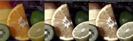
现在,你已经学习了最基本的知识。 这里 你将会看到一个混合使用C接口和C++接口的例子。你也可以在可以再OpenCV的代码库中的sample目录中找到此文件samples/cpp/tutorial_code/core/interoperability_with_OpenCV_1/interoperability_with_OpenCV_1.cpp 。为了进一步帮助你认清其中区别,程序支持两种模式:C和C++混合,以及纯C++。如果你宏定义了 DEMO_MIXED_API_USE ,程序将按第一种模式编译。程序的功能是划分颜色平面,对其进行改动并最终将其重新合并。

 1
 2
 3
 4
 5
 6
 7
 8
 9
10
11
12
13
14
15
16
17
18
19
20
21
22
23
24
25
26
27
28
29
30
31
#include 
#include 

#include 
#include 
#include 

using namespace cv;  // The new C++ interface API is inside this namespace. Import it.
using namespace std;
#define DEMO_MIXED_API_USE 

int main( int argc, char** argv )
{
    const char* imagename = argc > 1 ? argv[1] : "lena.jpg";

#ifdef DEMO_MIXED_API_USE
    Ptr<IplImage> IplI = cvLoadImage(imagename);      // Ptr is safe ref-counting pointer class
    if(IplI.empty())
    {
        cerr << "Can not load image " <<  imagename << endl;
        return -1;
    }
    Mat I(IplI); // Convert to the new style container. Only header created. Image not copied.    
#else
    Mat I = imread(imagename);        // the newer cvLoadImage alternative, MATLAB-style function
    if( I.empty() )                   // same as if( !I.data )
    {
        cerr << "Can not load image " <<  imagename << endl;
        return -1;
    }
#endif

在此,你可一看到新的结构再无指针问题,哪怕使用旧的函数,并在最后结束时将结果转换为 Mat 对象。

1
2
3
4
5
6
    // convert image to YUV color space. The output image will be created automatically. 
    Mat I_YUV;
    cvtColor(I, I_YUV, CV_BGR2YCrCb); 

    vector<Mat> planes;    // Use the STL's vector structure to store multiple Mat objects 
    split(I_YUV, planes);  // split the image into separate color planes (Y U V)

因为我们打算搞乱图像的亮度通道,所以首先将图像由默认的RGB颜色空间转为YUV颜色空间,然后将其划分为独立颜色平面(Y,U,V)。第一个例子中,我们对每一个平面用OpenCV中三个主要图像扫描算法(C []操作符,迭代,单独元素访问)中的一个进行处理。在第二个例子中,我们给图像添加一些高斯噪声,然后依据一些准则融合所有通道。

运用扫描算法的代码如下:

 1
 2
 3
 4
 5
 6
 7
 8
 9
10
11
12
13
14
15
16
17
18
19
20
21
    // Method 1. process Y plane using an iterator
    MatIterator_<uchar> it = planes[0].begin<uchar>(), it_end = planes[0].end<uchar>();
    for(; it != it_end; ++it)
    {
        double v = *it * 1.7 + rand()%21 - 10;
        *it = saturate_cast<uchar>(v*v/255);
    }
    
    for( int y = 0; y < I_YUV.rows; y++ )
    {
        // Method 2. process the first chroma plane using pre-stored row pointer.
        uchar* Uptr = planes[1].ptr<uchar>(y);
        for( int x = 0; x < I_YUV.cols; x++ )
        {
            Uptr[x] = saturate_cast<uchar>((Uptr[x]-128)/2 + 128);
            
            // Method 3. process the second chroma plane using individual element access
            uchar& Vxy = planes[2].at<uchar>(y, x);
            Vxy =        saturate_cast<uchar>((Vxy-128)/2 + 128);
        }
    }

此处可看到,我们可以以三种方式遍历图像的所有像素:迭代器,C指针和单独元素访问方式你可在 OpenCV如何扫描图像、利用查找表和计时 中获得更深入的了解。从旧的函数名转换新版本非常容易,仅需要删除 cv 前缀,并且使用 Mat 数据结构。下面的例子中使用了加权加法:

 1
 2
 3
 4
 5
 6
 7
 8
 9
10
11
12
13
14
15
16
17
18
19
20
21
22
23
24
25
26
27
28
29
30
31
32
33
34
    Mat noisyI(I.size(), CV_8U);           // Create a matrix of the specified size and type
    
    // Fills the matrix with normally distributed random values (around number with deviation off).
    // There is also randu() for uniformly distributed random number generation
    randn(noisyI, Scalar::all(128), Scalar::all(20)); 
    
    // blur the noisyI a bit, kernel size is 3x3 and both sigma's are set to 0.5
    GaussianBlur(noisyI, noisyI, Size(3, 3), 0.5, 0.5); 

    const double brightness_gain = 0;
    const double contrast_gain = 1.7;

#ifdef DEMO_MIXED_API_USE
    // To pass the new matrices to the functions that only work with IplImage or CvMat do:
    // step 1) Convert the headers (tip: data will not be copied).
    // step 2) call the function   (tip: to pass a pointer do not forget unary "&" to form pointers)
    
    IplImage cv_planes_0 = planes[0], cv_noise = noisyI;    
    cvAddWeighted(&cv_planes_0, contrast_gain, &cv_noise, 1, -128 + brightness_gain, &cv_planes_0);
#else
    addWeighted(planes[0], contrast_gain, noisyI, 1, -128 + brightness_gain, planes[0]);
#endif
    
    const double color_scale = 0.5;
    // Mat::convertTo() replaces cvConvertScale. 
    // One must explicitly specify the output matrix type (we keep it intact - planes[1].type())
    planes[1].convertTo(planes[1], planes[1].type(), color_scale, 128*(1-color_scale));

    // alternative form of cv::convertScale if we know the datatype at compile time ("uchar" here).
    // This expression will not create any temporary arrays ( so should be almost as fast as above)
    planes[2] = Mat_<uchar>(planes[2]*color_scale + 128*(1-color_scale));

    // Mat::mul replaces cvMul(). Again, no temporary arrays are created in case of simple expressions.
    planes[0] = planes[0].mul(planes[0], 1./255);

正如你所见,变量 planes 也是 Mat 类型的。无论如何,将 Mat 转换为 IplImage 都可通过简单的赋值操作符自动实现。

 1
 2
 3
 4
 5
 6
 7
 8
 9
10
11
12
13
    
    merge(planes, I_YUV);                // now merge the results back
    cvtColor(I_YUV, I, CV_YCrCb2BGR);  // and produce the output RGB image

    
    namedWindow("image with grain", CV_WINDOW_AUTOSIZE);   // use this to create images

#ifdef DEMO_MIXED_API_USE
    // this is to demonstrate that I and IplI really share the data - the result of the above
    // processing is stored in I and thus in IplI too.
    cvShowImage("image with grain", IplI);
#else
    imshow("image with grain", I); // the new MATLAB style function show

新的 imshow highgui函数可接受 Mat 和 IplImage 数据结构。 编译并运行例程,如果输入以下第一幅图像,程序将输出以下第二幅或者第三幅图像。

OpenCV之core 模块. 核心功能(2)基本绘图 随机数发生器&绘制文字 离散傅立叶变换 输入输出XML和YAML文件 与 OpenCV 1 同时使用_第7张图片

你可以在点击此处看到动态示例: YouTube here ,并可以 点击此处 下载源文件,或者在OpenCV源代码库中找到源文件:samples/cpp/tutorial_code/core/interoperability_with_OpenCV_1/interoperability_with_OpenCV_1.cpp 。


from: http://www.opencv.org.cn/opencvdoc/2.3.2/html/doc/tutorials/core/table_of_content_core/table_of_content_core.html#table-of-content-core

你可能感兴趣的:(OpenCV,OpenCV,core,模块,核心功能,绘图,离散傅立叶变换)