Pandas中DataFrame的属性、方法、常用操作以及使用示例

---

前言

系列文章目录
[Python]目录
视频及资料和课件
链接：https://pan.baidu.com/s/1LCv_qyWslwB-MYw56fjbDg?pwd=1234
提取码：1234

---

---

包的引入：

import numpy as np
import pandas as pd

1. DataFrame 对象创建

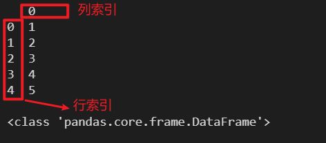
1.1 通过列表创建 DataFrame 对象

l = [1, 2, 3, 4, 5]
df = pd.DataFrame(l)
print(df)
print()
print(type(df))

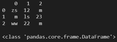
l = [
  ['zs', 12, 'm'],
  ['ls', 23, 'm'],
  ['ww', 22, 'm']
]
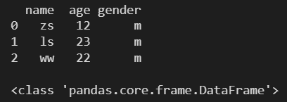
df1 = pd.DataFrame(l)
print(df1)
print()
print(type(df1))
print()

l = [
  {'zs', 12, 'm'},
  {'ls', 23, 'm'},
  {'ww', 22, 'm'}
]
df1 = pd.DataFrame(l)
print(df1)
print()
print(type(df1))
print()

由于集合是无序的，所以创建的 DataFrame 对象中元素的顺序也无序。

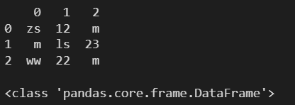
1.2 通过元组创建 DataFrame 对象

t = (1, 2, 3, 4, 5)
df = pd.DataFrame(t)
print(df)
print()
print(type(df))

l = (
  ['zs', 12, 'm'],
  ['ls', 23, 'm'],
  ['ww', 22, 'm']
)
df1 = pd.DataFrame(l)
print(df1)
print()
print(type(df1))
print()

l = (
  {'zs', 12, 'm'},
  {'ls', 23, 'm'},
  {'ww', 22, 'm'}
)
df1 = pd.DataFrame(l)
print(df1)
print()
print(type(df1))
print()

1.3 通过集合创建 DataFrame 对象

集合内不能嵌套集合、列表

s = {1, 2, 3, 4, 5, 2, 2, 5, 6}
df = pd.DataFrame(s)
print(df)
print()
print(type(df))

l = {
  ('zs', 12, 'm'),
  ('ls', 23, 'm'),
  ('ww', 22, 'm')
}
df1 = pd.DataFrame(
  l, 
  columns=['name', 'age', 'gender'], 
  index=['a', 'b', 'c'],
  dtype='float64'
)
print(df1)
print()
print(type(df1))
print()

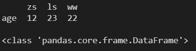
1.4 通过字典创建 DataFrame 对象

d = {
  'zs': 12,
  'ls': 23,
  'ww': 22
}
# 只有一层字典必须使用 index 指定索引
# index 指定的索引为行索引
# 字典的 key 为列索引
df = pd.DataFrame(d, index=['age'])
print(df)
print()
print(type(df))

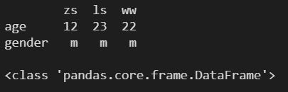
d = {
  'zs': {'age': 12, 'gender': 'm'},
  'ls': {'age': 23, 'gender': 'm'},
  'ww': {'age': 22, 'gender': 'm'}
}
# 多层字典不用使用 index 指定索引
# 外层字典的 key 为列索引
# 内层字典的 key 为行索引
df = pd.DataFrame(d)
print(df)
print()
print(type(df))

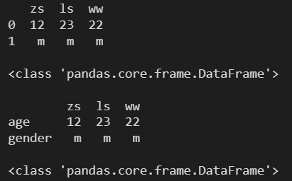
d = {
  'zs': [12, 'm'],
  'ls': [23, 'm'],
  'ww': [22, 'm']
}
df1 = pd.DataFrame(d)
print(df1)
print()
print(type(df1))
print()
df2 = pd.DataFrame(d, index=['age', 'gender'])
print(df2)
print()
print(type(df2))

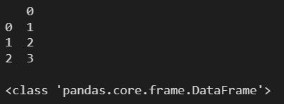
1.5 通过Series 对象创建 DataFrame 对象

l = pd.Series([1,2,3])
df = pd.DataFrame(l)
print(df)
print()
print(type(df))

l = [
  pd.Series([1,2,3]),
  pd.Series([4,5,6]),
  pd.Series([7,8,9])
]
df = pd.DataFrame(l)
print(df)
print()
print(type(df))

1.6 通过 ndarray 创建 DataFrame 对象

l = np.array([1,2,3])
df = pd.DataFrame(l)
print(df)
print()
print(type(df))

l = [
  np.array([1,2,3]),
  np.array([4,5,6]),
  np.array([7,8,9])
]
df = pd.DataFrame(l)
print(df)
print()
print(type(df))

1.7 创建 DataFrame 对象时指定列索引

• columns：指定列索引

l = [
  ['zs', 12, 'm'],
  ['ls', 23, 'm'],
  ['ww', 22, 'm']
]
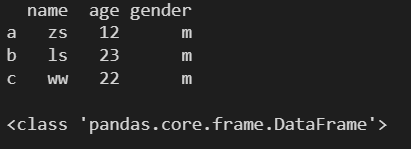
df1 = pd.DataFrame(l, columns=['name', 'age', 'gender'])
print(df1)
print()
print(type(df1))
print()

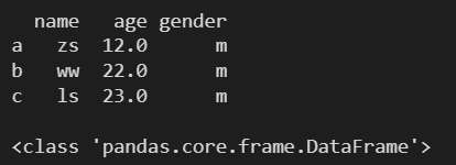
1.8 创建 DataFrame 对象时指定行索引

• index：指定行索引

l = [
  ['zs', 12, 'm'],
  ['ls', 23, 'm'],
  ['ww', 22, 'm']
]
df1 = pd.DataFrame(
  l, 
  columns=['name', 'age', 'gender'], 
  index=['a', 'b', 'c']
)
print(df1)
print()
print(type(df1))
print()

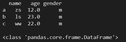
1.9 创建 DataFrame 对象时指定元素的数据类型

• dtype：指定元素的数据类型

字符串数据类型的数据元素会被忽略

l = [
  ['zs', 12, 'm'],
  ['ls', 23, 'm'],
  ['ww', 22, 'm']
]
df1 = pd.DataFrame(
  l, 
  columns=['name', 'age', 'gender'], 
  index=['a', 'b', 'c'],
  dtype='float64'
)
print(df1)
print()
print(type(df1))
print()

1.10 创建 DataFrame 对象的注意点

使用列表创建 DataFrame 对象时，不同列表的长度不同会报错。

data = {
    'one': [1,2,3],
    'two': [1,2,3,4],
}
df = pd.DataFrame(data)

ValueError: All arrays must be of the same length

使用 Series 对象创建 DataFrame 对象，不同长度不同会报错。

data = {
    'one': pd.Series([1,2,3]),
    'two': pd.Series([1,2,3,4]),
}
df = pd.DataFrame(data)
print(df)

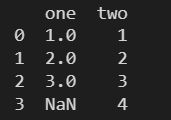
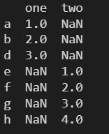
Series 可以保证列数据个数不一样的不同列的各行数据元素位置相对应

data = {
    'one': pd.Series([1, 2, 3], index=['a', 'b', 'd']),
    'two': pd.Series([1, 2, 3, 4], index=['a', 'b', 'c', 'd']),
}
df = pd.DataFrame(data)
print(df)

data = {
    'one': pd.Series([1, 2, 3], index=['a', 'b', 'd']),
    'two': pd.Series([1, 2, 3, 4], index=['e', 'f', 'g', 'h']),
}
df = pd.DataFrame(data)
print(df)

2. DataFrame 的属性

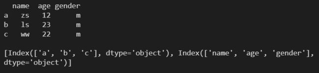
2.1 axes ---- 返回行/列标签列表

l = [
  ['zs', 12, 'm'],
  ['ls', 23, 'm'],
  ['ww', 22, 'm']
]
df1 = pd.DataFrame(
  l, 
  columns=['name', 'age', 'gender'], 
  index=['a', 'b', 'c']
)
print(df1)
print()
print(df1.axes)

2.2 columns ---- 返回列标签列表

l = [
  ['zs', 12, 'm'],
  ['ls', 23, 'm'],
  ['ww', 22, 'm']
]
df1 = pd.DataFrame(
  l, 
  columns=['name', 'age', 'gender'], 
  index=['a', 'b', 'c']
)
print(df1)
print()
print(df1.columns)

2.3 index ---- 返回行标签列表

l = [
  ['zs', 12, 'm'],
  ['ls', 23, 'm'],
  ['ww', 22, 'm']
]
df1 = pd.DataFrame(
  l, 
  columns=['name', 'age', 'gender'], 
  index=['a', 'b', 'c']
)
print(df1)
print()
print(df1.index)

2.4 dtypes ---- 返回数据类型

l = [
  ['zs', 12, 'm'],
  ['ls', 23, 'm'],
  ['ww', 22, 'm']
]
df1 = pd.DataFrame(
  l, 
  columns=['name', 'age', 'gender'], 
  index=['a', 'b', 'c']
)
print(df1)
print()
print(df1.dtypes)

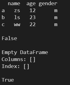
2.5 empty ---- 返回 DataFrame 对象是否为空

l = [
  ['zs', 12, 'm'],
  ['ls', 23, 'm'],
  ['ww', 22, 'm']
]
df1 = pd.DataFrame(
  l, 
  columns=['name', 'age', 'gender'], 
  index=['a', 'b', 'c']
)
print(df1)
print()
print(df1.empty)
print()
df2 = pd.DataFrame()
print(df2)
print()
print(df2.empty)

2.6 ndim ---- 返回 DateFrame 对象的维数

l = [
  ['zs', 12, 'm'],
  ['ls', 23, 'm'],
  ['ww', 22, 'm']
]
df1 = pd.DataFrame(
  l, 
  columns=['name', 'age', 'gender'], 
  index=['a', 'b', 'c']
)
print(df1)
print()
print(df1.ndim)

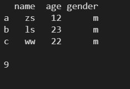
2.7 size ---- 返回DateFrame 对象中的数据元素个数

l = [
  ['zs', 12, 'm'],
  ['ls', 23, 'm'],
  ['ww', 22, 'm']
]
df1 = pd.DataFrame(
  l, 
  columns=['name', 'age', 'gender'], 
  index=['a', 'b', 'c']
)
print(df1)
print()
print(df1.size)

2.8 values ---- 返回数据元素组成的 ndarray 数组

l = [
  ['zs', 12, 'm'],
  ['ls', 23, 'm'],
  ['ww', 22, 'm']
]
df1 = pd.DataFrame(
  l, 
  columns=['name', 'age', 'gender'], 
  index=['a', 'b', 'c']
)
print(df1)
print()
print(df1.values)

2.9 shape ---- 返回 DataFrame 对象的维度

l = [
  ['zs', 12, 'm'],
  ['ls', 23, 'm'],
  ['ww', 22, 'm']
]
df1 = pd.DataFrame(
  l, 
  columns=['name', 'age', 'gender'], 
  index=['a', 'b', 'c']
)
print(df1)
print()
print(df1.shape)

2.10 T ---- 返回 DataFrame 对象的转置

l = [
  pd.Series([1,2,3]),
  pd.Series([4,5,6]),
  pd.Series([7,8,9])
]
df = pd.DataFrame(l)
print(df)
print()
print(df.T)

3. DataFrame 的方法

3.1 head() ---- 返回 DataFrame 对象的前 x 行

默认前五行

l = [
  ['zs', 12, 'm'],
  ['ls', 23, 'm'],
  ['ww', 22, 'm']
]
df1 = pd.DataFrame(
  l, 
  columns=['name', 'age', 'gender'], 
  index=['a', 'b', 'c']
)
print(df1)
print()
print(df1.head(1))

3.2 tail() ---- 返回 DataFrame 对象的后 x 行

默认后五行

l = [
  ['zs', 12, 'm'],
  ['ls', 23, 'm'],
  ['ww', 22, 'm']
]
df1 = pd.DataFrame(
  l, 
  columns=['name', 'age', 'gender'], 
  index=['a', 'b', 'c']
)
print(df1)
print()
print(df1.tail(1))

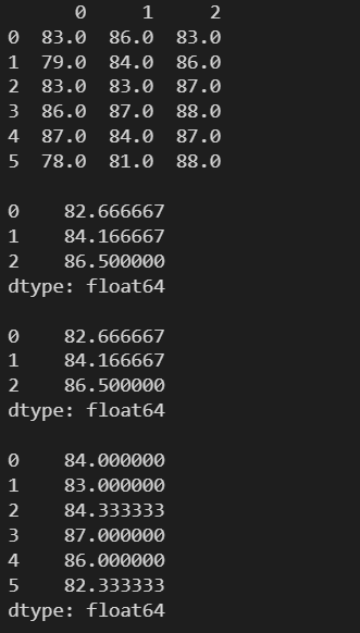
3.3 mean() ---- 求算术平均数

# 生成一个 6 行 3 列的数组
data = np.floor(np.random.normal(85, 3, (6,3)))
df = pd.DataFrame(data)
print(df)
print()
# 默认计算每列的算数平均数
print(df.mean())
print()
# axis 可以指定计算的方向，默认 axis=0 计算每列的算数平均数
print(df.mean(axis=0))
print()
# 计算每行的算数平均数
print(df.mean(axis=1))
print()

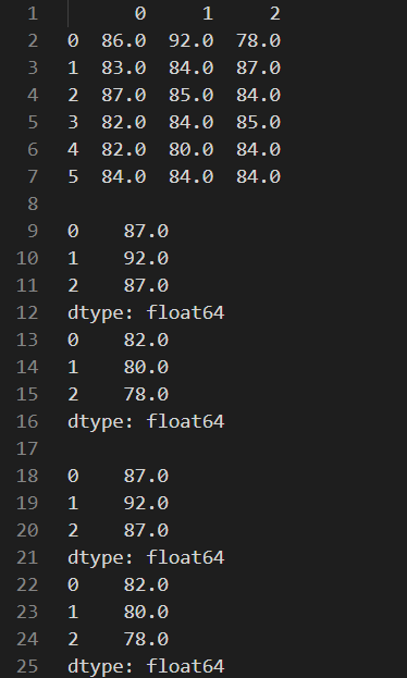
3.4 min() max() ---- 求最值

# 生成一个 6 行 3 列的数组
data = np.floor(np.random.normal(85, 3, (6,3)))
df = pd.DataFrame(data)
print(df)
print()
# 默认计算每列的最值
print(df.max())
print(df.min())
print()
# axis 可以指定计算的方向，默认 axis=0 计算每列的最值
print(df.max(axis=0))
print(df.min(axis=0))
print()
# 计算每行的算数平均数
print(df.max(axis=1))
print(df.min(axis=1))
print()

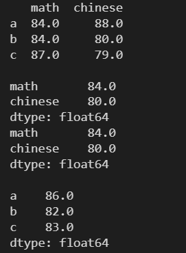
3.5 idxmax() idxmin() ---- 获取最值索引

data = np.floor(np.random.normal(85, 3, (3,2)))
df = pd.DataFrame(data, index=['a', 'b', 'c'], columns=['math', 'chinese'])
print(df)
print()
# 列
print(df.max(), df.idxmax())
print()
print(df.min(), df.idxmin())
print()
# 行
print(df.max(axis=1), df.idxmax(axis=1))
print()
print(df.min(axis=1), df.idxmin(axis=1))

3.6 median() ---- 求中位数

data = np.floor(np.random.normal(85, 3, (3,2)))
df = pd.DataFrame(data, index=['a', 'b', 'c'], columns=['math', 'chinese'])
print(df)
print()
# 列
print(df.median())
print(df.median(axis=0))
print()
# 行
print(df.median(axis=1))

3.7 value_counts() ---- 求频数

以行为统计单元

data = np.floor(np.random.normal(85, 3, (3,2)))
df = pd.DataFrame(data, index=['a', 'b', 'c'], columns=['math', 'chinese'])
print(df)
print()
print(df.value_counts())

3.8 mode() ---- 求众数

data = np.floor(np.random.normal(85, 3, (3,2)))
df = pd.DataFrame(data, index=['a', 'b', 'c'], columns=['math', 'chinese'])
print(df)
print()
print(df.mode())
print()
print(df.mode(axis=1))

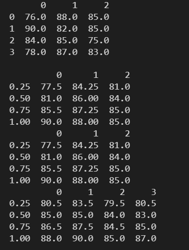
3.9 quantile() ---- 求四分位数

四分位数：把数值从小到大排列并分成四等分，处于三个分割点位置的数值就是四分位数。

• 需要传入一个列表，列表中的元素为要获取的数的对应位置

data = np.floor(np.random.normal(85, 3, (4,3)))
df = pd.DataFrame(data)
print(df)
print()
print(df.quantile([.25, .50, .75, 1]))
print(df.quantile([.25, .50, .75, 1], axis=0))
print(df.quantile([.25, .50, .75, 1], axis=1))

3.10 std() ---- 标准差

总体标准差是反映研究总体内个体之间差异程度的一种统计指标。
总体标准差计算公式：
$S=\sqrt{\frac{\sum {\left(X_i-\bar{X}\right)}^2}{n}}$

由于总体标准差计算出来会偏小，所以采用$(n-ddof)$的方式适当扩大标准差，即样本标准差。
样本标准差计算公式：
$S=\sqrt{\frac{\sum {\left(X_i-\bar{X}\right)}^2}{n-ddof}}$

data = np.floor(np.random.normal(85, 3, (4,3)))
df = pd.DataFrame(data)
print(df)
print()
# 总体标准差
print(df.std())
print(df.std(axis=0))
print(df.std(axis=1))

data = np.floor(np.random.normal(85, 3, (4,3)))
df = pd.DataFrame(data)
print(df)
print()
# 样本标准差
print(df.std(ddof=1))
print(df.std(axis=0,ddof=1))
print(df.std(axis=1,ddof=1))

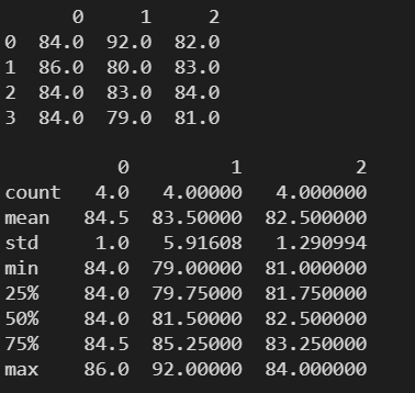
3.11 describe() ---- 统计 DataFrame 的常见统计学指标结果

data = np.floor(np.random.normal(85, 3, (4,3)))
df = pd.DataFrame(data)
print(df)
print()
print(df.describe())

3.12 corr() ---- 求每列之间的相关系数矩阵

相关系数：描述两组样本的相关程度的大小
相关系数：协方差除去两组样本标准差的乘积，是一个 [-1, 1] 之间的数

data = np.floor(np.random.normal(85, 3, (4,3)))
df = pd.DataFrame(data)
print(df)
print()
print(df.corr())

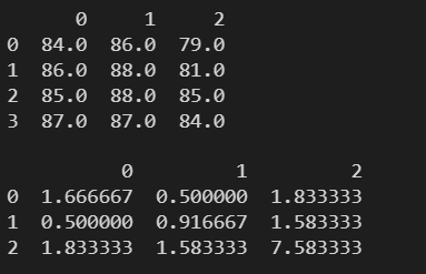
3.12 cov() ---- 求每列之间的协方差矩阵

协方差：可以评估两组统计数据的相关性
协方差正为正相关，负为反相关。绝对值越大，相关性越强。
计算方法：

1. 计算两组样本的均值
2. 计算两组样本中的各个元素与均值的差
3. 协方差为 两组数据离差的乘积的均值

data = np.floor(np.random.normal(85, 3, (4,3)))
df = pd.DataFrame(data)
print(df)
print()
print(df.cov())

3.13 sort_values() ---- 根据元素值进行排序

参数：

• by：指定排序参照的字段
• ascending：True为升序(默认)，False为降序
• axis：排序的方向， 0 - 对行进行排序(默认)，1 - 对列进行排序

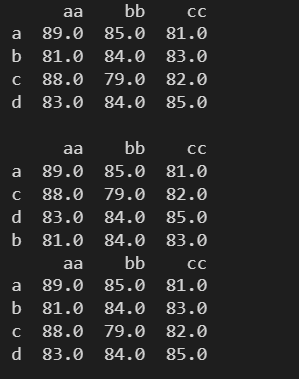
3.13.1 升序

data = np.floor(np.random.normal(85, 3, (4,3)))
df = pd.DataFrame(data, index=['a','b','c','d'], columns=['aa','bb','cc'])
print(df)
print()
# 根据 aa 列对数据进行升序排列
print(df.sort_values(by=['aa']))
# 根据 a 行对数据进行升序排列
print(df.sort_values(by=['a'],axis=1))
# 根据 a 行对数据进行升序排列
print(df.sort_values(by=['a'],axis=1, ascending=True))

3.13.2 降序

data = np.floor(np.random.normal(85, 3, (4,3)))
df = pd.DataFrame(data, index=['a','b','c','d'], columns=['aa','bb','cc'])
print(df)
print()
# 根据 aa 列对数据进行降序排列
print(df.sort_values(by=['aa'], ascending=False))
# 根据 a 行对数据进行降序排列
print(df.sort_values(by=['a'],axis=1, ascending=False))

3.14 sort_index() ---- 根据索引值进行排序

参数：

• ascending：True为升序(默认)，False为降序
• axis：排序的方向， 0 - 对行进行排序(默认)，1 - 对列进行排序

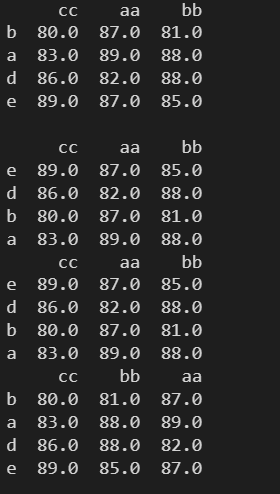
3.14.2 升序

data = np.floor(np.random.normal(85, 3, (4,3)))
df = pd.DataFrame(data, index=['b','a','d','e'], columns=['cc','aa','bb'])
print(df)
print()
# 默认对行索引进行升序排列
print(df.sort_index())
# 对行索引进行升序排列
print(df.sort_index(axis=0))
# 对列索引进行升序排列
print(df.sort_index(axis=1))

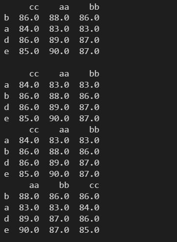
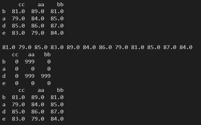
3.14.2 降序

data = np.floor(np.random.normal(85, 3, (4,3)))
df = pd.DataFrame(data, index=['b','a','d','e'], columns=['cc','aa','bb'])
print(df)
print()
# 默认对行索引进行降序排列
print(df.sort_index(ascending=False))
# 对行索引进行降序排列
print(df.sort_index(axis=0,ascending=False))
# 对列索引进行降序排列
print(df.sort_index(axis=1,ascending=False))

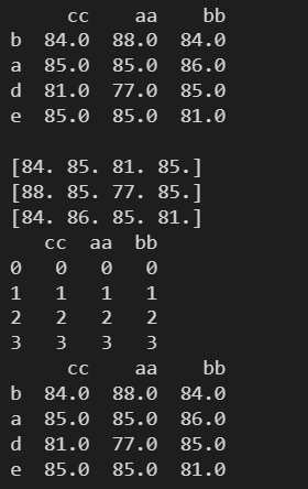
3.15 apply() ---- 根据传入的函数参数处理 DataFrame 对象

3.15.1 对每列进行处理

def func(x):
  print(x.values)
  return pd.Series(np.arange(0,x.size))

data = np.floor(np.random.normal(85, 3, (4,3)))
df = pd.DataFrame(data, index=['b','a','d','e'], columns=['cc','aa','bb'])
print(df)
print()
# 默认对每列进行处理，一次处理一列
# 会返回一个原数组处理后的新数组，不会修改原数组
res = df.apply(func)
print(res)
print(df)

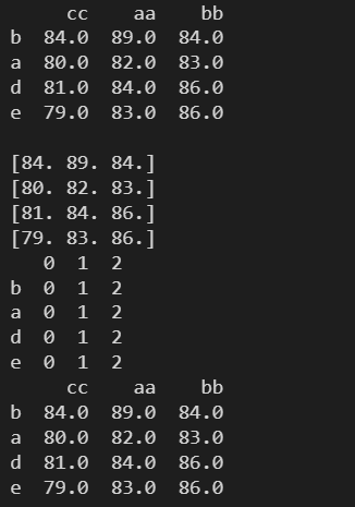
3.15.2 对每行进行处理

def func(x):
  print(x.values)
  return pd.Series(np.arange(0,x.size))

data = np.floor(np.random.normal(85, 3, (4,3)))
df = pd.DataFrame(data, index=['b','a','d','e'], columns=['cc','aa','bb'])
print(df)
print()
res = df.apply(func, axis=1)
print(res)
print(df)

3.16 applymap() ---- 根据传入的函数参数处理 DataFrame 对象的每个元素

按列的方向遍历每个元素进行处理，返回一个处理后的新数组，不会修改原数组。

def func(x):
  print(x, end=' ')
  if(x>85): return 999
  else: return 0

data = np.floor(np.random.normal(85, 3, (4,3)))
df = pd.DataFrame(data, index=['b','a','d','e'], columns=['cc','aa','bb'])
print(df)
print()
res = df.applymap(func)
print()
print(res)
print(df)

3.17 groupby() ---- 对 DataFrame 对象中的数据进行分组

参数：

• by：指定分组的依据，可以接收的参数类型 list、string、mapping、generator
• axis：操作的轴向，默认对行进行操作，默认为0，接收
• as_index：表示聚合后的聚合标签是否以DataFrame索引形式输出，默认为True
• sort：表示是否对分组依据分组标签进行排序，默认为True

返回 Groupby 对象：

• Groupby.get_group(‘A’)：返回A组的详细数据
• Groupby.size()：返回每一组的频数

数据：

left = pd.DataFrame({
         'student_id':[1,2,3,4,5,6,7,8,9,10,11,12,13,14,15,16,17,18,19,20],
         'student_name': ['Alex', 'Amy', 'Allen', 'Alice', 'Ayoung', 'Billy', 'Brian', 'Bran', 'Bryce', 'Betty', 'Emma', 'Marry', 'Allen', 'Jean', 'Rose', 'David', 'Tom', 'Jack', 'Daniel', 'Andrew'],
         'class_id':[1,1,1,2,2,2,3,3,3,4,1,1,1,2,2,2,3,3,3,2], 
         'gender':['M', 'M', 'F', 'F', 'M', 'M', 'F', 'F', 'M', 'M', 'F', 'F', 'M', 'M', 'F', 'F', 'M', 'M', 'F', 'F'], 
         'age':[20,21,22,20,21,22,23,20,21,22,20,21,22,23,20,21,22,20,21,22], 
         'score':[98,74,67,38,65,29,32,34,85,64,52,38,26,89,68,46,32,78,79,87]})
left
right = pd.DataFrame({'class_id':[1,2,3,5],  'class_name': ['ClassA', 'ClassB', 'ClassC', 'ClassE']})
right
data = pd.merge(left, right, how='inner', on='class_id')

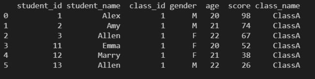
3.17.1 分组

# 根据 class_id 进行分组
grouped = data.groupby(by='class_id')
# 获取 class_id 为1的组
print(grouped.get_group(1))

# 根据 class_id 与 gender 进行分组
grouped = data.groupby(by=['class_id', 'gender'])
# # 获取 class_id gender 为(1, 'M')的组
print(grouped.get_group((1, 'M')))

print(grouped.size())

3.17.1 聚合

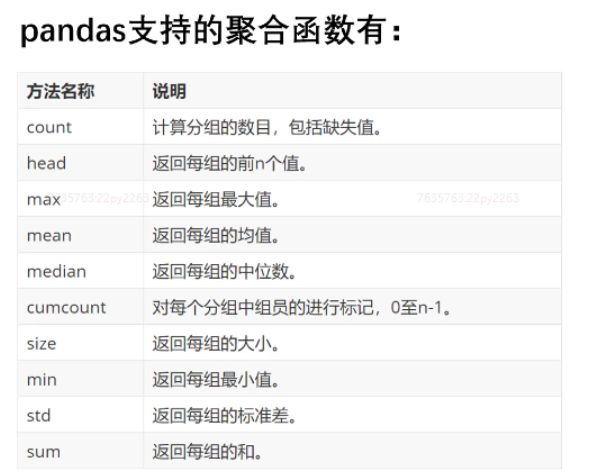
# 根据 class_id 进行分组
grouped = data.groupby(by='class_id')
# 统计每个班级的平均分
# 传入的字典对应的值为处理的方式
print(grouped.agg({'score': np.mean}))

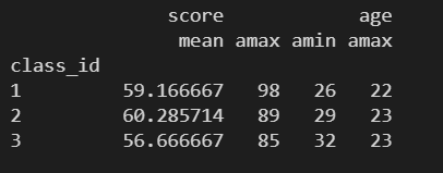
# 统计每个班级的平均分, 以及么每个班级的年龄最大值
print(grouped.agg({'score':np.mean, 'age':np.max}))

print(grouped.agg({'score':[np.mean, np.max, np.min], 'age':np.max}))

3.18 pivot_table() ---- 生成DataFrame对象的透视表

参数：

• index：分组所依据的列
• values：指定需要聚合统计的列
• columns：指定列，依据该列的每个值进行分列统计
• margins：是否对透视表的每行每列进行汇总统计
• aggfunc：聚合要执行的操作

# 根据 class_id 进行分组
# 默认求分组后能进行均值计算的列的均值
print(data.pivot_table(index='class_id') )

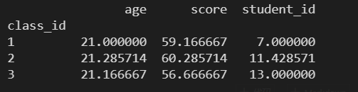
# 根据 class_id 进行分组
# 对分组后的数据 score 的聚合操作，默认求均值
print(data.pivot_table(index='class_id', values='score') )

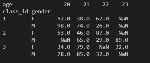
# 根据 class_id gender 进行分组
# 对分组后的数据 score 的聚合操作，默认求均值
# 依据 age 列的每个值进行分列统计
print(
  data.pivot_table(
    index=['class_id', 'gender'], 
    values='score', 
    columns=['age']
  )
)

# 根据 class_id gender 进行分组
# 对分组后的数据 score 的聚合操作，默认求均值
# 依据 age 列的每个值进行分列统计
# 对透视表的每行每列进行汇总统
print(
  data.pivot_table(
    index=['class_id', 'gender'], 
    values='score', 
    columns=['age'], 
    margins=True
  )
)

print(
  data.pivot_table(
    index=['class_id', 'gender'], 
    values='score', 
    columns=['age'], 
    margins=True,
    aggfunc='max'
  )
)

3.19 drop_duplicates ---- 处理重复值

属性：

• subset：接收 string 或 序列 为参数，表示要进行去重的列，默认为None，表示全部的列(只有当一行中所有的列一样，才会对该行进行去重)
• keep：接收 string 为参数，表示重复时保留第几个数据。first：保留第一个。last：保留最后一个。false：只要有重复都不保留。默认为first。
• inplace：表示是否在原表上进行修改。默认为False。

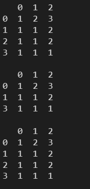
默认情况下，对所有的列进行去重，不在原表上进行修改，有重复值时默认保留重复值的第一个。

l = [
  np.array([1,2,3]),
  np.array([1,1,2]),
  np.array([1,1,2]),
  np.array([1,1,1])
]
df = pd.DataFrame(l)
print(df)
print()
print(df.drop_duplicates())
print()
print(df)

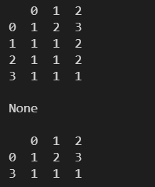
l = [
  np.array([1,2,3]),
  np.array([1,1,2]),
  np.array([1,1,2]),
  np.array([1,1,1])
]
df = pd.DataFrame(l)
print(df)
print()
# 在原表上进行修改，无返回值
# 不在原表上进行修改，会返回修改后的新表
print(df.drop_duplicates(subset=[0,1], inplace=True, keep='last'))
print()
print(df)

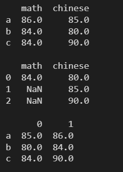
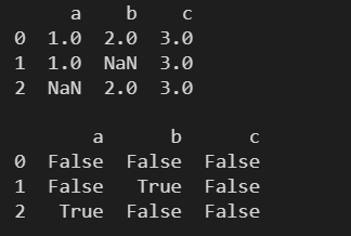
3.20 isnull() ---- 判断是否为缺失值

l = [
  pd.Series([1,2,3], index=['a', 'b', 'c']),
  pd.Series([1,3], index=['a', 'c']),
  pd.Series([2,3], index=['b', 'c'])
]
df = pd.DataFrame(l)
print(df)
print()
print(df.isnull())

3.21 notnull() ---- 判断是否不为缺失值

l = [
  pd.Series([1,2,3], index=['a', 'b', 'c']),
  pd.Series([1,3], index=['a', 'c']),
  pd.Series([2,3], index=['b', 'c'])
]
df = pd.DataFrame(l)
print(df)
print()
print(df.notnull())

3.22 sum() ---- 求和

l = [
  pd.Series([1,2,3], index=['a', 'b', 'c']),
  pd.Series([1,3], index=['a', 'c']),
  pd.Series([2,3], index=['b', 'c'])
]
df = pd.DataFrame(l)
print(df)
print()
# 默认对每列进行求和
print(df.sum())
# 对每列进行求和
print(df.sum(axis=0))
print()
# 对每行进行求和
print(df.sum(axis=1))

3.23 dropna() ---- 删除缺失值

参数：

• axis：表示轴向，0为删除行，1为删除列，默认为0.
• how：接收 string 为参数，表示删除的方式，any 表示只要有缺失值就删除该行或列，all表示全部为缺失值才删除行或列。默认为any。
• subset：接收 array 类型的数据为参数，表示进行缺失值处理的行或列，默认为None，表示所有的行或列。
• inplace：表示是否在原表上进行操作，默认为False。

l = [
  pd.Series([1,2,3], index=['a', 'b', 'c']),
  pd.Series([1,3], index=['a', 'c']),
  pd.Series([2,3], index=['b', 'c'])
]
df = pd.DataFrame(l)
print(df)
print()
# 默认执行删除行操作，只要有缺失值就执行删除操作
# 默认对所有的列进行处理
# 默认不在原表上进行修改
print(df.dropna())
print()
print(df)

l = [
  pd.Series([1,2,3], index=['a', 'b', 'c']),
  pd.Series([1,3], index=['a', 'c']),
  pd.Series([2,3], index=['b', 'c'])
]
df = pd.DataFrame(l)
print(df)
print()
# 有缺失值时删除列
# 对第三行进行处理
# 在原表上进行修改，不在原表上进行修改会返回修改后的新表
# 有缺失值就进行删除
print(df.dropna(axis=1, subset=[2], inplace=True, how='any'))
print()
print(df)

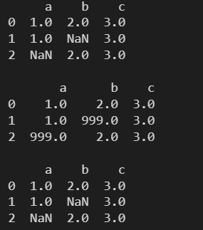
3.24 fillna() ---- 替换缺失值

参数：

• value：表示用来替换缺失值的值
• method：接收 string 为参数，backfill或bfill表示使用下一个非缺失值进行替换，pad或ffill表示使用上一个非缺失值进行替换，默认为None
• axis：表示轴向
• inplace：表示是否在原表上进行操作，默认为False。
• limit：表示填补缺失值的个数上限，默认为None
• value与method选择其一即可

l = [
  pd.Series([1,2,3], index=['a', 'b', 'c']),
  pd.Series([1,3], index=['a', 'c']),
  pd.Series([2,3], index=['b', 'c'])
]
df = pd.DataFrame(l)
print(df)
print()
# 使用 999 填补缺失值
# 不在原表进行修改
print(df.fillna(999))
print()
print(df)

l = [
  pd.Series([1,2,3], index=['a', 'b', 'c']),
  pd.Series([1,3], index=['a', 'c']),
  pd.Series([2,3], index=['b', 'c'])
]
df = pd.DataFrame(l)
print(df)
print()
# 使用后一个非缺失值进行填补
# 轴向为列，使用后一列的非缺失值进行填补
# 在原表上进行修改
print(df.fillna(method='bfill', axis=1, inplace=True))
print()
print(df)

3.25 info() ---- 获取 DataFrame 中数据的简要摘要

df = pd.read_excel('./数据文件/信表节点的坐标.xlsx')
df.info()

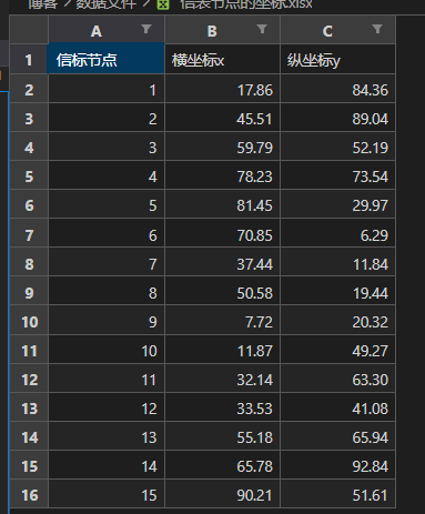
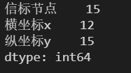
3.26 count() ---- 统计每列中不为空的值的个数

df = pd.read_excel('./数据文件/信表节点的坐标.xlsx')
df.count()

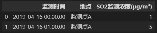
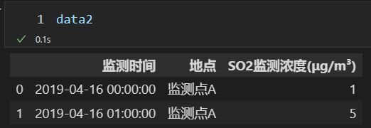
3.27 copy() ---- 对DateFrame对象进行复制

参数：
deep：deep=True，表示进行深复制；deep=False，表示进行浅复制。默认为 True。

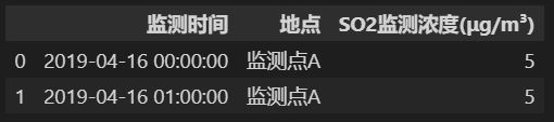
data1 = data.iloc[0:2, 0:3]
data2 = data1.copy()
data2['SO2监测浓度(μg/m³)'][0] = 1
data1

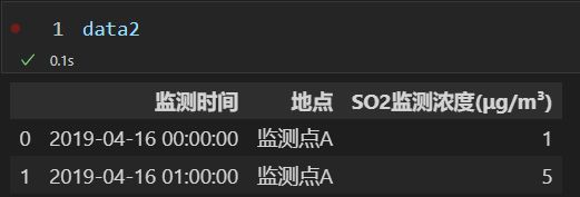
data1 = data.iloc[0:2, 0:3]
data2 = data1.copy(deep=False)
data2['SO2监测浓度(μg/m³)'][0] = 1
data1

4. DataFrame 的常用操作

4.1 列的访问

DataFrame 的单列数据为一个 Series 。根据 DataFrame 的定义，DataFrame 是一个带有标签的二维数组，每个标签相当于每一列的列名。

4.1.1 根据标签索引进行访问

l = [
  ['zs', 12, 'm'],
  ['ls', 23, 'm'],
  ['ww', 22, 'm']
]
df1 = pd.DataFrame(
  l, 
  columns=['name', 'age', 'gender'], 
  index=['a', 'b', 'c']
)
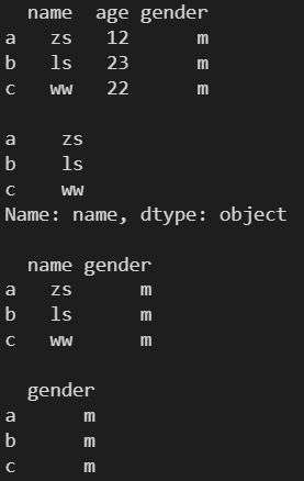
print(df1)
print()
print(df1['name'])
print()
# 注意为 嵌套列表
print(df1[['name', 'gender']])

4.1.2 根据数字索引进行访问

l = [
  ['zs', 12, 'm'],
  ['ls', 23, 'm'],
  ['ww', 22, 'm']
]
df1 = pd.DataFrame(
  l, 
  columns=['name', 'age', 'gender'], 
  index=['a', 'b', 'c']
)
print(df1)
print()
print(df1[df1.columns[0]])
print()
print(df1[df1.columns[0:3:2]])
print()
print(df1[df1.columns[-1:0:-2]])

4.2 列的添加

DataFrame 添加列，只需要新建一个列索引，并对该索引下的数据进行赋值操作即可。

l = [
  ['zs', 12],
  ['ls', 23],
  ['ww', 22]
]
df1 = pd.DataFrame(
  l, 
  columns=['name', 'age'], 
  index=['a', 'b', 'c']
)
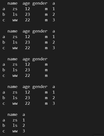
print(df1)
print()
# Series 需要设置索引
df1['gender'] = pd.Series(['m','m','m'], index=['a', 'b', 'c'])
print(df1)
df1['a'] = [1, 2, 3]
print(df1)

4.3 列的删除

删除某列数据，需要用 pandas 提供的方法 pop 或 drop 方法。

4.3.1 pop()

l = [
  ['zs', 12],
  ['ls', 23],
  ['ww', 22]
]
df1 = pd.DataFrame(
  l, 
  columns=['name', 'age'], 
  index=['a', 'b', 'c']
)
df1['gender'] = pd.Series(['m','m','m'], index=['a', 'b', 'c'])
df1['a'] = [1, 2, 3]
print(df1)
print()
# 返回删除的列
# 一次只能删除一列，对原数组进行修改
res = df1.pop('a')
print(df1)
print()
print(res)

4.3.2 drop()

l = [
  ['zs', 12],
  ['ls', 23],
  ['ww', 22]
]
df1 = pd.DataFrame(
  l, 
  columns=['name', 'age'], 
  index=['a', 'b', 'c']
)
df1['gender'] = pd.Series(['m','m','m'], index=['a', 'b', 'c'])
df1['a'] = [1, 2, 3]
print(df1)
print()
# drop 不对原数组进行修改，会返回一个新数组
# 支持多列删除
# axis 指定删除列还是行 列(1) 行(0)
# axis 默认取值为 0
res = df1.drop('a', axis=1)
print(df1)
print()
print(res)
print()
res = df1.drop(['age', 'gender'], axis=1)
print(df1)
print()
print(res)

4.4 行的访问

4.4.1 通过索引进行访问

l = [
  ['zs', 12, 'm'],
  ['ls', 23, 'm'],
  ['ww', 22, 'm']
]
df1 = pd.DataFrame(
  l, 
  columns=['name', 'age', 'gender'], 
  index=['a', 'b', 'c']
)
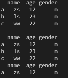
print(df1)
print()
# print(df1['a']) 对列进行访问， 访问列, ‘a’ 列不存在 会报错
print(df1['a':'c'])
# print(df1[0]) #对列进行访问， 访问列, 0 列不存在 会报错
print(df1[0:1])

4.4.2 loc()

loc() 是针对索引名称的访问方法

l = [
  ['zs', 12, 'm'],
  ['ls', 23, 'm'],
  ['ww', 22, 'm']
]
df1 = pd.DataFrame(
  l, 
  columns=['name', 'age', 'gender'], 
  index=['a', 'b', 'c']
)
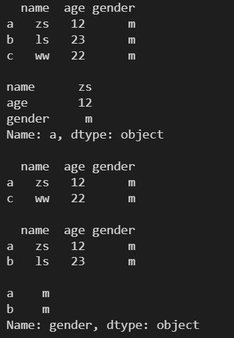
print(df1)
print()
# 访问 a 行
print(df1.loc['a'])
print()
# 访问 a c 行
print(df1.loc[['a', 'c']])
print()
# 访问 a 到 b 行(包含起始位置)
print(df1.loc['a':'b'])
print()
# loc[行，列]
print(df1.loc['a':'b', 'gender'])

4.4.3 iloc()

iloc() 是针对数字索引的访问方法

l = [
  ['zs', 12, 'm'],
  ['ls', 23, 'm'],
  ['ww', 22, 'm']
]
df1 = pd.DataFrame(
  l, 
  columns=['name', 'age', 'gender'], 
  index=['a', 'b', 'c']
)
print(df1)
print()
# 第 0 行
print(df1.iloc[0])
print()
# 第 0 2 行
print(df1.iloc[[0, 2]])
print()
# 第 0 到第 1 行
print(df1.iloc[0:2])
print()
# iloc[行，列]
# 第 0 1 行，第 1 列
print(df1.iloc[0:2, 1:2])

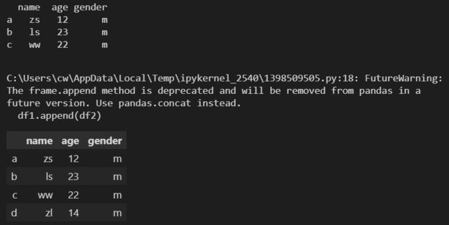
4.5 行的添加

使用 append() 方法进行添加

l = [
  ['zs', 12, 'm'],
  ['ls', 23, 'm'],
  ['ww', 22, 'm']
]
df1 = pd.DataFrame(
  l, 
  columns=['name', 'age', 'gender'], 
  index=['a', 'b', 'c']
)
print(df1)
print()
df2 = pd.DataFrame(['zl', 14, 'm'])
df1.append(df2)

需要指定列名与行的索引名

l = [
  ['zs', 12, 'm'],
  ['ls', 23, 'm'],
  ['ww', 22, 'm']
]
df1 = pd.DataFrame(
  l, 
  columns=['name', 'age', 'gender'], 
  index=['a', 'b', 'c']
)
print(df1)
print()
df2 = pd.DataFrame([['zl', 14, 'm']])
df1.append(df2)

l = [
  ['zs', 12, 'm'],
  ['ls', 23, 'm'],
  ['ww', 22, 'm']
]
df1 = pd.DataFrame(
  l, 
  columns=['name', 'age', 'gender'], 
  index=['a', 'b', 'c']
)
print(df1)
print()
df2 = pd.DataFrame(
  [['zl', 14, 'm']], 
  columns=['name', 'age', 'gender'], 
  index=['d']
)
df1.append(df2)

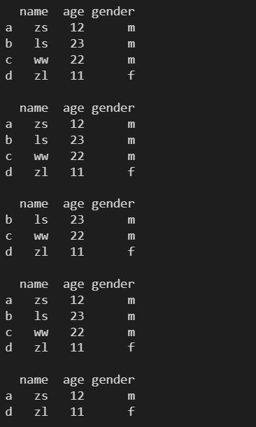
4.6 行的删除

调用 drop 方法通过索引标签删除行，标签重复会删除多行。

l = [
  ['zs', 12, 'm'],
  ['ls', 23, 'm'],
  ['ww', 22, 'm'],
  ['zl', 11, 'f']
]
df1 = pd.DataFrame(
  l, 
  columns=['name', 'age', 'gender'], 
  index=['a', 'b', 'c', 'd']
)
print(df1)
print()
res = df1.drop('a')
print(df1)
print()
print(res)
print()
res = df1.drop(['b', 'c'], axis=0)
print(df1)
print()
print(res)

4.7 复合索引

DataFrame 的行索引和列索引都支持为复合索引，表示从不同角度记录数据。

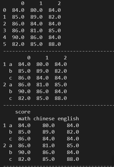
4.7.1 设置复合索引

# 生成一个 6 行 3 列的数组
data = np.floor(np.random.normal(85, 3, (6,3)))
df = pd.DataFrame(data)
print(df)
print('-'*50)

# 设置行的复合索引
index = [(1, 'a'), (1, 'b'), (1, 'c'), (2, 'a'), (2, 'b'), (2, 'c')]
df.index = pd.MultiIndex.from_tuples(index)
print(df)
print('-'*50)

# 设置列的复合索引
column = [('score', 'math'), ('score', 'chinese'), ('score', 'english')]
df.columns = pd.MultiIndex.from_tuples(column)
print(df)
print('-'*50)

4.7.2 复合索引的访问

# 访问行
# 访问行索引为 1
print(df.loc[1])
print()
# 不同级之间的索引使用逗号进行分割
# 访问行索引为 (1, 'a')
print(df.loc[1, 'a'])
print()

# 访问行与列
# 访问行索引为 (1, 'a'); 列索引为 ('score', 'math')
print(df.loc[1, 'a']['score','math'])
print()

# 同级索引访问多个
# 访问行索引为 (1, 'a') (1, 'b'), (2, 'a') (2, 'b'); 
# 列索引为 ('score', 'math') ('score', 'chinese') 
# 注意 行 列 索引要使用元组
# 行：([1, 2], ['a', 'b'])
# 行索引 第一级   第二级
# 列：('score', ['math', 'chinese'])
# 列索引 第一级   第二级
print(df.loc[([1, 2], ['a', 'b']), ('score', ['math', 'chinese'])])