arima 预测模型_预测未来：学习使用Arima模型进行预测

arima 预测模型

XTS对象 (XTS Objects)

If you’re not using XTS objects to perform your forecasting in R, then you are likely missing out! The major benefits that we’ll explore throughout are that these objects are a lot easier to work with when it comes to modeling, forecasting, & visualization.

如果您没有使用XTS对象在R中执行预测，那么您很可能会错过！ 我们将始终探索的主要好处是，在建模，预测和可视化方面，这些对象更易于使用。

让我们进入细节 (Let’s Get to The Details)

XTS objects are composed of two components. The first is a date index and the second of which is a traditional data matrix.

XTS对象由两个组件组成。 第一个是日期索引，第二个是传统数据矩阵。

Whether you want to predict churn, sales, demand, or whatever else, let’s get to it!

无论您是要预测客户流失，销售，需求还是其他，我们都可以开始吧！

The first thing you’ll need to do is create your date index. We do so using the seq function. Very simply this function takes what is your start date, the number of records you have or length, and then the time interval or by parameter. For us, the dataset starts with the following.

您需要做的第一件事是创建日期索引。 我们使用seq函数。 很简单，此功能需要的只是你的开始日期，你有记录的数目或长度，然后将时间间隔或by参数。 对于我们来说，数据集从以下开始。

days <- seq(as.Date("2014-01-01"), length = 668, by = "day")

Now that we have our index, we can use it to create our XTS object. For this, we will use the xts function.

现在我们有了索引，可以使用它来创建XTS对象。 为此，我们将使用xts函数。

Don’t forget to install.packages('xts') and then load the library! library(xts)

不要忘了先安装install.packages('xts') ，然后加载库！ library(xts)

Once we’ve done this we’ll make our xts call and pass along our data matrix, and then for the date index we will pass the index to the order.by option.

完成此操作后，我们将进行xts调用并传递数据矩阵，然后对于日期索引，我们会将索引传递给order.by选项。

sales_xts <- xts(sales, order.by = days)

让我们与Arima建立预测 (Let’s Create a Forecast with Arima)

Arima stands for auto regressive integrated moving average. A very popular technique when it comes to time series forecasting. We could spend hours talking about ARIMA alone, but for this post, we’re going to give a high-level explanation and then jump directly into the application.

有马代表自动回归综合移动平均线。 关于时间序列预测的一种非常流行的技术。 我们可能只花几个小时来谈论ARIMA，但是在这篇文章中，我们将给出一个高级的解释，然后直接进入该应用程序。

AR：自回归 (AR: Auto Regressive)

This is where we predict outcomes using lags or values from previous months. It may be that the outcomes of a given month have some dependency on previous values.

在这里，我们使用前几个月的滞后或值来预测结果。 给定月份的结果可能与以前的值有一定的依赖性。

一：集成 (I: Integrated)

When it comes to time series forecasting, an implicit assumption is that our model depends on time in some capacity. This seems pretty obvious as we probably wouldn’t make our model time based otherwise ;). With that assumption out of the way, we need to understand where on the spectrum of dependence time falls in relation to our model. Yes, our model depends on time, but how much? Core to this is the idea of Stationarity; which means that the effect of time diminishes as time goes on.

在进行时间序列预测时，一个隐含的假设是我们的模型在某种程度上取决于时间。 这似乎很明显，因为我们可能不会将模型时间设为其他时间；)。 有了这个假设，我们需要了解与我们的模型有关的依赖时间范围。 是的，我们的模型取决于时间，但是多少？ 核心思想是平稳性 ； 这意味着随着时间的流逝，时间的影响减弱。

Going deeper, the historical average of a dataset tends to be the best predictor of future outcomes… but there are certainly times when that’s not true.. can you think of any situations when the historical mean would not be the best predictor?

更深入地讲，数据集的历史平均值往往是未来结果的最佳预测因子……但是，在某些情况下，这是不正确的……您能想到历史均值不是最佳预测因子的任何情况吗？

• How about predicting sales for December? Seasonal Trends
  预测12月的销售情况如何？ 季节性趋势
• How about sales for a hyper-growth saas company? Consistent upward trends
  一家高速增长的saas公司的销售情况如何？ 一致的上升趋势

This is where the process of Differencing is introduced! Differencing is used to eliminate the effects of trends & seasonality.

这就是引入差分过程的地方！ 差异用于消除趋势和季节性的影响。

MA：移动平均线 (MA: Moving Average)

the moving average model exists to deal with the error of your model.

存在移动平均模型以处理模型误差。

让我们开始建模吧！ (Let’s Get Modeling!)

火车/验证拆分 (Train/Validation Split)

First things first, let’s break out our data into a training dataset and then what we’ll call our validation dataset.

首先，让我们将数据分为训练数据集，然后将其称为验证数据集。

What makes this different than other validation testing, like cross-validation testing is that here we break it out by time, breaking train up to a given point in time and breaking out validation for everything thereafter.

与其他验证测试(例如交叉验证测试)不同的是，这里我们按时间细分，将训练分解到给定的时间点，然后对所有内容进行验证。

train <- sales_xts[index(sales_xts) <= "2015-07-01"] 
validation <- sales_xts[index(sales_xts) > "2015-07-01"]

是时候建立模型了 (Time to Build a Model)

The auto.arima function incorporates the ideas we just spoke about to approximate the best arima model. I will detail the more hands-on approach in another post, but below I’ll explore the generation of an auto.arima model and how to use it to forecast.

auto.arima函数结合了我们刚才谈到的想法，可以近似最佳arima模型。 我将在另一篇文章中详细介绍更多的动手方法，但是下面我将探讨auto.arima模型的生成以及如何使用它进行预测。

model <- auto.arima(train)

Now let’s generate a forecast. The same way we did before, we’ll create a date index and then create an xts object with the data matrix.

现在让我们生成一个预测。 与之前相同，我们将创建一个日期索引，然后使用数据矩阵创建一个xts对象。

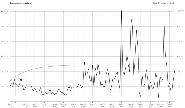
From here you will plot the validation data and then throw the forecast on top of the plot.

在这里，您将绘制验证数据，然后将预测放在该图的顶部。

forecast <- forecast(model, h = 121) 
forecast_dates <- seq(as.Date("2015-09-01"), length = 121, by = "day")forecast_xts <- xts(forecast$mean, order.by = forecast_dates)plot(validation, main = 'Forecast Comparison')lines(forecast_xts, col = "blue")

结论 (Conclusion)

I hope this was a helpful introduction to ARIMA forecasting. Be sure to let me know what’s helpful and any additional detail you’d like to learn about.

我希望这对ARIMA预测很有帮助。 请务必让我知道有什么帮助以及您想了解的任何其他详细信息。

If you found this helpful be sure to check out some of my other posts on datasciencelessons.com. Happy Data Science-ing!

如果您认为这有帮助，请务必在datasciencelessons.com上查看我的其他一些帖子。 快乐数据科学！

翻译自: https://towardsdatascience.com/predicting-the-future-learn-to-forecast-with-arima-models-879853c46a4d

arima 预测模型