鲍鱼数据集 岭回归解析解

要求：首先数据集进行一定的预处理，之后计算岭回归的解析解，并采用合适的指标对结果进行评估。

import pandas as pd
import warnings
warnings.filterwarnings('ignore')#忽略匹配警告
data=pd.read_csv(r'C:/Users/86139/Desktop/大二下/机器学习/机器学习实践/abalone_dataset.csv')
data.head()

	sex	length	diameter	height	whole weight	shucked weight	viscera weight	shell weight	rings
0	M	0.455	0.365	0.095	0.5140	0.2245	0.1010	0.150	15
1	M	0.350	0.265	0.090	0.2255	0.0995	0.0485	0.070	7
2	F	0.530	0.420	0.135	0.6770	0.2565	0.1415	0.210	9
3	M	0.440	0.365	0.125	0.5160	0.2155	0.1140	0.155	10
4	I	0.330	0.255	0.080	0.2050	0.0895	0.0395	0.055	7

一、预处理

#2.1对sex特征进行onehot编码，便于后续模型纳入哑变量
sex_onehot=pd.get_dummies(data['sex'],prefix="sex")
data[sex_onehot.columns]=sex_onehot
data.head()

	sex	length	diameter	height	whole weight	shucked weight	viscera weight	shell weight	rings	sex_F	sex_I	sex_M
0	M	0.455	0.365	0.095	0.5140	0.2245	0.1010	0.150	15	0	0	1
1	M	0.350	0.265	0.090	0.2255	0.0995	0.0485	0.070	7	0	0	1
2	F	0.530	0.420	0.135	0.6770	0.2565	0.1415	0.210	9	1	0	0
3	M	0.440	0.365	0.125	0.5160	0.2155	0.1140	0.155	10	0	0	1
4	I	0.330	0.255	0.080	0.2050	0.0895	0.0395	0.055	7	0	1	0

#2.2添加取值为1的特征
data["ones"]=1
data.head()

	sex	length	diameter	height	whole weight	shucked weight	viscera weight	shell weight	rings	sex_F	sex_I	sex_M	ones
0	M	0.455	0.365	0.095	0.5140	0.2245	0.1010	0.150	15	0	0	1	1
1	M	0.350	0.265	0.090	0.2255	0.0995	0.0485	0.070	7	0	0	1	1
2	F	0.530	0.420	0.135	0.6770	0.2565	0.1415	0.210	9	1	0	0	1
3	M	0.440	0.365	0.125	0.5160	0.2155	0.1140	0.155	10	0	0	1	1
4	I	0.330	0.255	0.080	0.2050	0.0895	0.0395	0.055	7	0	1	0	1

#2.3根据鲍鱼环计算年龄。
#一般每过一年，鲍鱼就会在其壳上留下一道深深的印记，这叫生长纹，就相当于树木的年轮。在本数据集中，我们要预测的是鲍鱼的年龄，可以通过环数rings 加上1.5得到。
data['age']=data['rings']+1.5
data.head()

	sex	length	diameter	height	whole weight	shucked weight	viscera weight	shell weight	rings	sex_F	sex_I	sex_M	ones	age
0	M	0.455	0.365	0.095	0.5140	0.2245	0.1010	0.150	15	0	0	1	1	16.5
1	M	0.350	0.265	0.090	0.2255	0.0995	0.0485	0.070	7	0	0	1	1	8.5
2	F	0.530	0.420	0.135	0.6770	0.2565	0.1415	0.210	9	1	0	0	1	10.5
3	M	0.440	0.365	0.125	0.5160	0.2155	0.1140	0.155	10	0	0	1	1	11.5
4	I	0.330	0.255	0.080	0.2050	0.0895	0.0395	0.055	7	0	1	0	1	8.5

#2.4筛选特征
#将预测目标设置为 age列，然后构造两组特征，一组包含ones，一组不包含ones。对于 sex相关的列，我们只使用sex_F和sex_M。
y=data['age']#因变量
features_with_ones=[ 'length', 'diameter', 'height', 'whole weight', 'shucked weight',
       'viscera weight', 'shell weight',  'sex_F', 'sex_M','ones']
features_without_ones=[ 'length', 'diameter', 'height', 'whole weight', 'shucked weight',
       'viscera weight', 'shell weight', 'sex_F', 'sex_M']
X=data[features_with_ones]

#2.5 将鲍鱼数据集划分为训练集和测试集
#将数据集随机划分为训练集和测试集，其中80%样本为训练集，剩余20%样本为测试集。
from sklearn.model_selection import train_test_split
X_train,X_test,y_train,y_test=train_test_split(X,y,test_size=0.2,random_state=111)

二、计算岭回归解析解

(1)使用Numpy实现岭回归（Rigde）

def ridge_regression(X,y,ridge_lambda):
    penalty_matrix=np.eye(X.shape[1])
    penalty_matrix[X.shape[1]-1][X.shape[1]-1]=0
    w=np.linalg.inv(X.T.dot(X)+ridge_lambda*penalty_matrix).dot(X.T).dot(y)
    return w

import numpy as np
w2=ridge_regression(X_train,y_train,1.0)
w2

array([  2.30976528,   6.72038628,  10.23298909,   7.05879189,
       -17.16249532,  -7.2343118 ,   9.3936994 ,   0.96869974,
         0.9422174 ,   4.80583032])

w2=pd.DataFrame(data=w2,index=X.columns,columns=['numpy_ridge_w'])
w2['numpy_ridge_w']=w2
w2.round(decimals=2)

	numpy_ridge_w
length	2.31
diameter	6.72
height	10.23
whole weight	7.06
shucked weight	-17.16
viscera weight	-7.23
shell weight	9.39
sex_F	0.97
sex_M	0.94
ones	4.81

(2)利用sklearn实现岭回归

#与sklearn中岭回归对比，同样正则化系数设置为 1
from sklearn.linear_model import Ridge
#模型实例化
ridge=Ridge(alpha=1)
#模型训练
ridge.fit(X_train[features_without_ones],y_train)
w_ridge=[]
w_ridge.extend(ridge.coef_)#coef_权重向量
w_ridge.append(ridge.intercept_)#intercept_决策函数的独立项，即截距b值。如果fit_intercept = False，则设置为0.0。
w2["ridge_sklearn_w"]=w_ridge
w2.round(decimals=2)

	numpy_ridge_w	ridge_sklearn_w
length	2.31	2.31
diameter	6.72	6.72
height	10.23	10.23
whole weight	7.06	7.06
shucked weight	-17.16	-17.16
viscera weight	-7.23	-7.23
shell weight	9.39	9.39
sex_F	0.97	0.97
sex_M	0.94	0.94
ones	4.81	4.81

**

三、结果评估

**

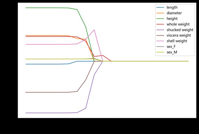
#岭迹分析
alpha=np.logspace(-10,10,20)
coef=pd.DataFrame()
for alpha in alpha:
    lasso_clf=Lasso(alpha=alpha)
    lasso_clf.fit(X_train[features_without_ones],y_train)
    df=pd.DataFrame([lasso_clf.coef_],columns=X_train[features_without_ones].columns)
    df['alpha']=alpha
    coef=coef.append(df,ignore_index=True)
coef.round(decimals=2)

	length	diameter	height	whole weight	shucked weight	viscera weight	shell weight	sex_F	sex_M	alpha
0	-1.12	10.00	20.74	9.61	-20.05	-12.07	6.55	0.88	0.87	0.000000e+00
1	-1.12	10.00	20.74	9.61	-20.05	-12.07	6.55	0.88	0.87	0.000000e+00
2	-1.12	10.00	20.74	9.61	-20.05	-12.07	6.55	0.88	0.87	0.000000e+00
3	-1.12	10.00	20.74	9.61	-20.05	-12.07	6.55	0.88	0.87	0.000000e+00
4	-1.11	9.99	20.73	9.61	-20.05	-12.07	6.55	0.88	0.87	0.000000e+00
5	-1.02	9.89	20.67	9.60	-20.04	-12.04	6.56	0.88	0.87	0.000000e+00
6	-0.00	8.76	20.02	9.46	-19.94	-11.72	6.73	0.88	0.88	0.000000e+00
7	0.00	8.56	13.35	7.78	-18.27	-7.28	8.52	0.90	0.89	0.000000e+00
8	0.00	0.00	0.00	1.84	-5.19	0.00	12.18	1.10	0.93	3.000000e-02
9	0.00	0.00	0.00	2.25	0.00	0.00	0.00	0.00	0.00	3.000000e-01
10	0.00	0.00	0.00	0.00	0.00	0.00	0.00	0.00	0.00	3.360000e+00
11	0.00	0.00	0.00	0.00	0.00	0.00	0.00	0.00	0.00	3.793000e+01
12	0.00	0.00	0.00	0.00	0.00	0.00	0.00	0.00	0.00	4.281300e+02
13	0.00	0.00	0.00	0.00	0.00	0.00	0.00	0.00	0.00	4.832930e+03
14	0.00	0.00	0.00	0.00	0.00	0.00	0.00	0.00	0.00	5.455595e+04
15	0.00	0.00	0.00	0.00	0.00	0.00	0.00	0.00	0.00	6.158482e+05
16	0.00	0.00	0.00	0.00	0.00	0.00	0.00	0.00	0.00	6.951928e+06
17	0.00	0.00	0.00	0.00	0.00	0.00	0.00	0.00	0.00	7.847600e+07
18	0.00	0.00	0.00	0.00	0.00	0.00	0.00	0.00	0.00	8.858668e+08
19	0.00	0.00	0.00	0.00	0.00	0.00	0.00	0.00	0.00	1.000000e+10

import matplotlib.pyplot as plt
%matplotlib inline
#plt.rcParams['font.sans-serif']=['SimHei','Times New Roman']
plt.rcParams['font.sans-serif']=['Microsoft YaHei']
plt.rcParams['axes.unicode_minus']=False

plt.rcParams['figure.dpi']=200#分辨率
plt.figure(figsize=(9,6))
coef['alpha']=coef['alpha']

for feature in X_train.columns[:-1]:
    plt.plot('alpha',feature,data=coef)
ax=plt.gca()
ax.set_xscale('log')
plt.legend(loc='upper right')
plt.xlabel(r'$\alpha$',fontsize=15)
plt.ylabel('系数',fontsize=15)

Text(0, 0.5, '系数')

回归模型的评价指标

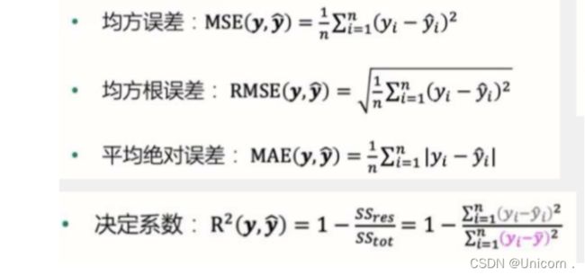
鲍鱼年龄预测模型效果评价

from sklearn.metrics import mean_squared_error
from sklearn.metrics import mean_absolute_error
from sklearn.metrics import r2_score

#MAE平均绝对误差
y_test_pred_ridge=ridge.predict(X_test[features_without_ones])
print(round(mean_absolute_error(y_test,y_test_pred_ridge),4))

#MSE 均方误差
y_test_pred_ridge=ridge.predict(X_test[features_without_ones])
print(round(mean_squared_error(y_test,y_test_pred_ridge),4))

#R^2系数
print(round(r2_score(y_test,y_test_pred_ridge),4))

1.5984
4.959
0.5563

残差图

残差图是一种用来诊断回归模型效果的图。在残差图中，如果点随机分布在0附近，则说明回归效果较好。如果在残差图中发现了某种结构，则说明回归效果不佳，需要重新建模。

plt.figure(figsize=(9,6),dpi=600)
y_train_pred_ridge=ridge.predict(X_train[features_without_ones])
plt.scatter(y_train_pred_ridge,y_train_pred_ridge-y_train,c='g',alpha=0.6)
plt.scatter(y_test_pred_ridge,y_test_pred_ridge-y_test,c='r',alpha=0.6)
plt.hlines(y=0,xmin=0,xmax=30,colors="b",alpha=0.6)
plt.ylabel('Residuals')
plt.xlabel('Predict')

Text(0.5, 0, 'Predict')