机器学习-线性回归（从零实现以及简化实现）

1、数据集的准备

如果有数据集，则跳过
生成一个包含1000个样本的数据集， 每个样本包含从标准正态分布中采样的2个特征 torch.normal(mean, std, size)
定义一个生成数据样本的函数

def get_data(w,b,num_examples):
	#使用正太分布均差为0，方差为1，生成大小（1000,2）
    X=torch.normal(0,1,(num_examples,len(w)))
    #矩阵相乘
    y=torch.matmul(X,w)+b
    #加上误差
    y+=torch.normal(0,0.01,y.shape)
    return X,y.reshape((-1,1))
#我们使用给定的w和b生成数据
#我们使用两个特征，要两个权重w
true_w=torch.tensor([2,-3.4])
true_b=4.2
features,labels=get_data(true_w,true_b,1000)
#把生成的数据拼接起来
features_labels=torch.cat([features,labels],dim=1)

2、保存到excel文件中

数据生成的为tensor数据类型，保存到excel文件中，要转换格式为numpy类型。

import numpy as np
import pandas as pd
 
# define a as the numpy array
data_excel = features_labels.numpy()
# transform a to pandas DataFrame
a_pd = pd.DataFrame(data_excel ,columns=['x1','x2','y'])
# create writer to write an excel file
writer = pd.ExcelWriter('a.xlsx')
# write in ro file, 'sheet1' is the page title, float_format is the accuracy of data
a_pd.to_excel(writer, 'sheet1', float_format='%.6f')
# save file
writer.save()

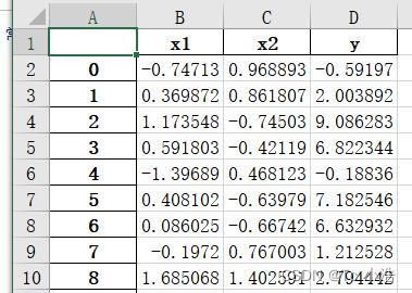
打开文件如下所示：

3、读取数据

读取文件的numpy数据格式

readbook = pd.read_excel(f'datas.xlsx', engine='openpyxl')
nplist = readbook.to_numpy()
data = nplist[0:]
data = np.float64(data)
#读取前两列
features_x=data[:,[0,1]]
#最后一列
target = data[:,[-1]]
#numpy转Tensor
features=torch.as_tensor(features,dtype=torch.float)
target=torch.as_tensor(target,dtype=float)

4、初始化模型参数

初始化模型参数，通过从均值为0、标准差为0.01的正态分布中采样随机数来初始化权重， 并将偏置初始化为0。

w=torch.normal(0,0.01,(2,1),requires_grad=True)
b=torch.zeros(1,requires_grad=True)

5、定义模型

$y=W^{T}X+b$

def liner(X,w,b):
    return torch.matmul(X,w)+b

6、定义损失函数

因为需要计算损失函数的梯度，所以我们应该先定义损失函数。

def loss(y_hat, y):  #@save
    """均方损失"""
    return (y_hat - y.reshape(y_hat.shape)) ** 2 / 2

7、定义优化算法

在每一步中，使用从数据集中随机抽取的一个小批量，然后根据参数计算损失的梯度。 接下来，朝着减少损失的方向更新我们的参数。 下面的函数实现小批量随机梯度下降更新。 该函数接受模型参数集合、学习速率和批量大小作为输入。每 一步更新的大小由学习速率lr决定。 因为我们计算的损失是一个批量样本的总和，所以我们用批量大小（batch_size） 来规范化步长，这样步长大小就不会取决于我们对批量大小的选择。

def sgd(params,lr,batch_size):
	#小批量随机梯度下降
	#使用with torch.no_grad():表明当前计算不需要反向传播，使用之后，强制后边的内容不进行计算图的构建
	with torch.no_grad():
		for param in params:
			param-=lr*param.grad/batch_size
			param.grad.zero_()

8、训练

lr = 0.03
num_epochs = 3
net = liner
loss = loss

for epoch in range(num_epochs):
    for X, y in data_iter(batch_size, features, labels):
        l = loss(net(X, w, b), y)  # X和y的小批量损失
        # 因为l形状是(batch_size,1)，而不是一个标量。l中的所有元素被加到一起，
        # 并以此计算关于[w,b]的梯度
        l.sum().backward()
        sgd([w, b], lr, batch_size)  # 使用参数的梯度更新参数
    with torch.no_grad():
        train_l = loss(net(features, w, b), labels)
        print(f'epoch {epoch + 1}, loss {float(train_l.mean()):f}')
       
#结果
epoch 1, loss 0.030909
epoch 2, loss 0.000110
epoch 3, loss 0.000053
epoch 4, loss 0.000053
epoch 5, loss 0.000053

因此我们通过训练得到了权重w和b

#输入特征进行预测
y_pred=torch.matmul(torch.tensor([[-0.74713,0.968893]]),w)+b
y_true=-59197
y_pred.item()=-0.5895