【slam十四讲第二版】【课本例题代码向】【第七讲~视觉里程计Ⅱ】【使用LK光流（cv）】【高斯牛顿法实现单层光流和多层光流】【实现单层直接法和多层直接法】

【slam十四讲第二版】【课本例题代码向】【第三~四讲刚体运动、李群和李代数】【eigen3.3.4和pangolin安装，Sophus及fim的安装使用】【绘制轨迹】【计算轨迹误差】

【slam十四讲第二版】【课本例题代码向】【第五讲~相机与图像】【OpenCV、图像去畸变、双目和RGB-D、遍历图像像素14种】

【slam十四讲第二版】【课本例题代码向】【第六讲~非线性优化】【安装对应版本ceres2.0.0和g2o教程】【手写高斯牛顿、ceres2.0.0、g2o拟合曲线及报错解决方案】
【slam十四讲第二版】【课本例题代码向】【第七讲~视觉里程计Ⅰ】【1OpenCV的ORB特征】【2手写ORB特征】【3对极约束求解相机运动】【4三角测量】【5求解PnP】【3D-3D:ICP】

0 前言

• 这一章节东西不多，希望快点学完
• 该章节所使用的数据集自取：链接: https://pan.baidu.com/s/1daebAx4DNHOtKrX8Up4lew 提取码: dcf5

1 使用LK光流（cv）

1.1 前言

• 这个部分仅仅涉及了如何配置cv中的LK函数的参数问题
• 其中所需要的数据集，以及我的工程包自取：链接：https://pan.baidu.com/s/1mlBdAiSiy2-jc23fYRyImg
  提取码：20dv

1.2 useLK.cpp

#include 
using namespace std;

#include 
#include 
#include 
#include 

#include 
#include 
#include 
#include 

int main(int argc, char** argv)
{
    string path_to_dataset;
    if (argc != 2)
    {
        path_to_dataset = "../data";
    }
    else
    {
        path_to_dataset = argv[1];
    }

    string associate_file = path_to_dataset + "/associate.txt";

    ifstream fin(associate_file);
    if (!fin)
    {
        cerr<<"I cann't find associate.txt!"<<endl;
        return 1;
    }

    string rgb_file, depth_file, time_rgb, time_depth;
    list< cv::Point2d > keypoints;// 因为要删除跟踪失败的点，使用list
    cv::Mat color, depth, last_color;

    for (int index = 0; index < 100; index++) {
        fin >> time_rgb >> rgb_file >> time_depth >> depth_file;
        color = cv::imread(path_to_dataset + "/" + rgb_file);//默认是IMREAD_COLOR = 1，彩色图
        depth = cv::imread(path_to_dataset + "/" + depth_file, -1);//-1 =IMREAD_UNCHANGED，深度图
        if (index == 0) {
            // 对第一帧提取FAST特征点
            vector<cv::KeyPoint> kps;
            cv::Ptr<cv::FastFeatureDetector> detector = cv::FastFeatureDetector::create();
            detector->detect(color, kps);
            for (auto kp: kps)
                keypoints.push_back(kp.pt);
            last_color = color;
            continue;
        }
        if (color.data == nullptr || depth.data == nullptr) continue;

        // 对其他帧用LK跟踪特征点
        vector<cv::Point2f> next_keypoints;
        vector<cv::Point2f> prev_keypoints;
        for (auto kp: keypoints)
            prev_keypoints.push_back(kp);
        vector<unsigned char> status;
        vector<float> error;
        chrono::steady_clock::time_point t1 = chrono::steady_clock::now();
        cv::calcOpticalFlowPyrLK( last_color, color, prev_keypoints, next_keypoints, status, error );
        chrono::steady_clock::time_point t2 = chrono::steady_clock::now();
        chrono::duration<double> time_used = chrono::duration_cast<chrono::duration<double>>( t2-t1 );
        cout<<"LK Flow use time："<<time_used.count()<<" seconds."<<endl;
        // 把跟丢的点删掉
        int i = 0;
        for (auto iter = keypoints.begin(); iter != keypoints.end(); i++) {
            if (status[i] == 0) {
                iter = keypoints.erase(iter);
                continue;
            }
            *iter = next_keypoints[i];
            iter++;
        }
        cout << "tracked keypoints: " << keypoints.size() << endl;
        if (keypoints.size() == 0) {
            cout << "all keypoints are lost." << endl;
            break;
        }

        // 画出 keypoints
        cv::Mat img_show = color.clone();
        for (auto kp: keypoints)
            cv::circle(img_show, kp, 10, cv::Scalar(0, 240, 0), 1);
        cv::imshow("corners", img_show);
        cv::waitKey(0);
        last_color = color;
    }
    return 0;
}

1.3 CMakeLists.txt

cmake_minimum_required(VERSION 2.8)

project(useLK)

set(CMAKE_BUILD_TYPE "Release")
set(CMAKE_CXX_STANDARD 14)

find_package(OpenCV 3 REQUIRED)

include_directories(${OpenCV_INCLUDE_DIRECTORIES})

add_executable(useLK src/useLK.cpp)

target_link_libraries(useLK ${OpenCV_LIBRARIES})

1.4 输出数据为

/home/bupo/shenlan/zuoye/cap8/useLK/cmake-build-release/useLK /home/bupo/shenlan/zuoye/cap8/useLK/data
LK Flow use time：0.0401681 seconds.
tracked keypoints: 1749
LK Flow use time：0.0229127 seconds.
tracked keypoints: 1742
LK Flow use time：0.0223572 seconds.
tracked keypoints: 1703
LK Flow use time：0.0220847 seconds.
tracked keypoints: 1676
LK Flow use time：0.0232433 seconds.
tracked keypoints: 1664
LK Flow use time：0.0211483 seconds.
tracked keypoints: 1656
LK Flow use time：0.0216098 seconds.
tracked keypoints: 1641
LK Flow use time：0.0220525 seconds.
tracked keypoints: 1634

进程已结束,退出代码0

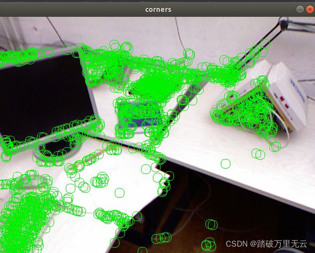
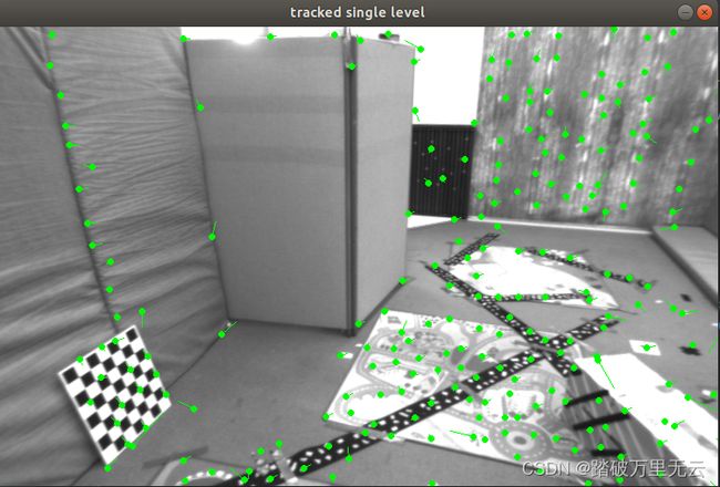
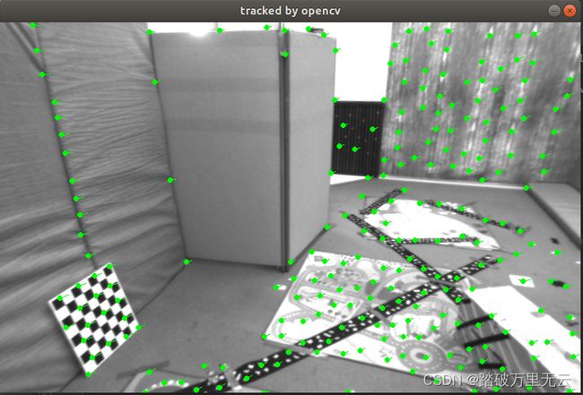
• 图片单张看并直观，最好亲身实践对比更为直观

1.5 感悟

• 暂无

2 高斯牛顿法实现单层光流和多层光流

2.1 前言

• 工程所必须的图片，以及我的实现工程自取：链接：https://pan.baidu.com/s/1CCNdyz1ozrX47z4s49CE5A
  提取码：gpjc

2.2 optical_flow.cpp

//
// Created by czy on 2022/4/10.
//

#include 
#include 
#include 
#include 
#include 

using namespace std;
using namespace cv;

string file_1 = "../src/LK1.png";  // first image
string file_2 = "../src/LK2.png";  // second image

/// Optical flow tracker and interface
class OpticalFlowTracker {
public:
    OpticalFlowTracker(
            const Mat &img1_,
            const Mat &img2_,
            const vector<KeyPoint> &kp1_,
            vector<KeyPoint> &kp2_,
            vector<bool> &success_,
            bool inverse_ = true,
            bool has_initial_ = false) :
            img1(img1_), img2(img2_), kp1(kp1_), kp2(kp2_), success(success_), inverse(inverse_),
            has_initial(has_initial_) {}

    void calculateOpticalFlow(const Range &range);

private:
    const Mat &img1;
    const Mat &img2;
    const vector<KeyPoint> &kp1;
    vector<KeyPoint> &kp2;
    vector<bool> &success;
    bool inverse = true;
    bool has_initial = false;
};

/**
 * single level optical flow
 * @param [in] img1 the first image
 * @param [in] img2 the second image
 * @param [in] kp1 keypoints in img1
 * @param [in|out] kp2 keypoints in img2, if empty, use initial guess in kp1
 * @param [out] success true if a keypoint is tracked successfully
 * @param [in] inverse use inverse formulation?
 */
void OpticalFlowSingleLevel(
        const Mat &img1,
        const Mat &img2,
        const vector<KeyPoint> &kp1,
        vector<KeyPoint> &kp2,
        vector<bool> &success,
        bool inverse = false,
        bool has_initial_guess = false
);

/**
 * multi level optical flow, scale of pyramid is set to 2 by default
 * the image pyramid will be create inside the function
 * @param [in] img1 the first pyramid
 * @param [in] img2 the second pyramid
 * @param [in] kp1 keypoints in img1
 * @param [out] kp2 keypoints in img2
 * @param [out] success true if a keypoint is tracked successfully
 * @param [in] inverse set true to enable inverse formulation
 */
void OpticalFlowMultiLevel(
        const Mat &img1,
        const Mat &img2,
        const vector<KeyPoint> &kp1,
        vector<KeyPoint> &kp2,
        vector<bool> &success,
        bool inverse = false
);

/**
 * get a gray scale value from reference image (bi-linear interpolated)
 * 从参考图像中获取灰度值(双线性插值)
 * @param img
 * @param x
 * @param y
 * @return the interpolated value of this pixel
 */
inline float GetPixelValue(const cv::Mat &img, float x, float y) {
    // boundary check
    if (x < 0) x = 0;
    if (y < 0) y = 0;
    if (x >= img.cols) x = img.cols - 1;
    if (y >= img.rows) y = img.rows - 1;
    uchar *data = &img.data[int(y) * img.step + int(x)];
    float xx = x - floor(x);
    float yy = y - floor(y);
    return float(
            (1 - xx) * (1 - yy) * data[0] +
            xx * (1 - yy) * data[1] +
            (1 - xx) * yy * data[img.step] +
            xx * yy * data[img.step + 1]
    );
}

int main(int argc, char **argv) {

    // images, note they are CV_8UC1, not CV_8UC3
    Mat img1 = imread(file_1, 0);//如果设置，总是将图像转换为单通道灰度图像。
    Mat img2 = imread(file_2, 0);

    // key points, using GFTT here.
    vector<KeyPoint> kp1;
    /*
     * 之前角点检测的算法中,一个是cornerHarris计算角点，但
     * 是这种角点检测算法容易出现聚簇现象以及角点信息有丢失和位置偏移现象，
     * 所以后面又提出一种名为goodFeatureToTrack的角点检测算法，
     * opencv的feature2D接口集成了这种算法,名称为 GFTTDetector。
     * */
    Ptr<GFTTDetector> detector = GFTTDetector::create(500, 0.01, 20); // maximum 500 keypoints
    detector->detect(img1, kp1);

    // now lets track these key points in the second image
    //现在让我们在第二张图中跟踪这些关键点
    // first use single level LK in the validation picture
    //首先在验证图中使用单级LK
    vector<KeyPoint> kp2_single;
    vector<bool> success_single;
    OpticalFlowSingleLevel(img1, img2, kp1, kp2_single, success_single);

    // then test multi-level LK然后测试多级LK，多层光流
    vector<KeyPoint> kp2_multi;
    vector<bool> success_multi;
    chrono::steady_clock::time_point t1 = chrono::steady_clock::now();
    OpticalFlowMultiLevel(img1, img2, kp1, kp2_multi, success_multi, true);
    chrono::steady_clock::time_point t2 = chrono::steady_clock::now();
    auto time_used = chrono::duration_cast<chrono::duration<double>>(t2 - t1);
    cout << "optical flow by gauss-newton: " << time_used.count() << endl;

    // use opencv's flow for validation
    vector<Point2f> pt1, pt2;
    for (auto &kp: kp1) pt1.push_back(kp.pt);
    vector<uchar> status;
    vector<float> error;
    t1 = chrono::steady_clock::now();
    cv::calcOpticalFlowPyrLK(img1, img2, pt1, pt2, status, error);
    t2 = chrono::steady_clock::now();
    time_used = chrono::duration_cast<chrono::duration<double>>(t2 - t1);
    cout << "optical flow by opencv: " << time_used.count() << endl;

    // plot the differences of those functions
    Mat img2_single;
    cv::cvtColor(img2, img2_single, CV_GRAY2BGR);
    for (int i = 0; i < kp2_single.size(); i++) {
        if (success_single[i]) {
            cv::circle(img2_single, kp2_single[i].pt, 2, cv::Scalar(0, 250, 0), 2);
            cv::line(img2_single, kp1[i].pt, kp2_single[i].pt, cv::Scalar(0, 250, 0));
        }
    }

    Mat img2_multi;
    cv::cvtColor(img2, img2_multi, CV_GRAY2BGR);
    for (int i = 0; i < kp2_multi.size(); i++) {
        if (success_multi[i]) {
            cv::circle(img2_multi, kp2_multi[i].pt, 2, cv::Scalar(0, 250, 0), 2);
            cv::line(img2_multi, kp1[i].pt, kp2_multi[i].pt, cv::Scalar(0, 250, 0));
        }
    }

    Mat img2_CV;
    cv::cvtColor(img2, img2_CV, CV_GRAY2BGR);
    for (int i = 0; i < pt2.size(); i++) {
        if (status[i]) {
            cv::circle(img2_CV, pt2[i], 2, cv::Scalar(0, 250, 0), 2);
            cv::line(img2_CV, pt1[i], pt2[i], cv::Scalar(0, 250, 0));
        }
    }

    cv::imshow("tracked single level", img2_single);
    cv::imshow("tracked multi level", img2_multi);
    cv::imshow("tracked by opencv", img2_CV);
    cv::waitKey(0);

    return 0;
}

void OpticalFlowSingleLevel(
        const Mat &img1,
        const Mat &img2,
        const vector<KeyPoint> &kp1,
        vector<KeyPoint> &kp2,
        vector<bool> &success,
        bool inverse, bool has_initial)
{
    kp2.resize(kp1.size());
    success.resize(kp1.size());
    OpticalFlowTracker tracker(img1, img2, kp1, kp2, success, inverse, has_initial);
    //Range表示一个范围，即并行计算哪些需要追踪的点,kp1中存放的就是随机选的追踪点
    //bind是一个绑定函数，它相当于调用OpticalFlowTracker.calculateOpticalFlow()，
    //std::placeholders::_1是占位符，表示传入的参数是OpticalFlowTracker.calculateOpticalFlow()的第一个参数，
    // 此处Range(0, kp1.size())为传入的参数。

    parallel_for_(Range(0, kp1.size()),
                  std::bind(&OpticalFlowTracker::calculateOpticalFlow, &tracker, placeholders::_1));
}

void OpticalFlowTracker::calculateOpticalFlow(const Range &range) {
    // parameters
    int half_patch_size = 4;
    int iterations = 10;
    for (size_t i = range.start; i < range.end; i++) {
        auto kp = kp1[i];
        double dx = 0, dy = 0; // dx,dy need to be estimated
        if (has_initial) {
            dx = kp2[i].pt.x - kp.pt.x;
            dy = kp2[i].pt.y - kp.pt.y;
        }

        double cost = 0, lastCost = 0;
        bool succ = true; // indicate if this point succeeded指示这一点是否成功

        // Gauss-Newton iterations
        Eigen::Matrix2d H = Eigen::Matrix2d::Zero();    // hessian
        Eigen::Vector2d b = Eigen::Vector2d::Zero();    // bias
        Eigen::Vector2d J;  // jacobian
        for (int iter = 0; iter < iterations; iter++)
        {
            /*
             * 这里是采用反向（Inverse）光流法。
             * 在反向的光流法中，可以使用第一个图像的像素梯度代替第二个像素的梯度
             * 在反向光流法中，第一个图像的向素梯度是不变的，所以可以保留第一次迭代的结果，在后续的迭代中使用
             * 当雅可比不变时，H矩阵不变，每次迭代只需计算残差，可以节省一部分计算量
             */
            if (inverse == false) {//
                H = Eigen::Matrix2d::Zero();
                b = Eigen::Vector2d::Zero();
            } else {
                // only reset b
                b = Eigen::Vector2d::Zero();
            }

            cost = 0;

            // compute cost and jacobian
            for (int x = -half_patch_size; x < half_patch_size; x++)
                for (int y = -half_patch_size; y < half_patch_size; y++)
                {
                    double error = GetPixelValue(img1, kp.pt.x + x, kp.pt.y + y) -
                                   GetPixelValue(img2, kp.pt.x + x + dx, kp.pt.y + y + dy);;  // Jacobian
                    if (inverse == false) {
                        J = -1.0 * Eigen::Vector2d(//求解像素的导数
                                0.5 * (GetPixelValue(img2, kp.pt.x + dx + x + 1, kp.pt.y + dy + y) -
                                       GetPixelValue(img2, kp.pt.x + dx + x - 1, kp.pt.y + dy + y)),
                                0.5 * (GetPixelValue(img2, kp.pt.x + dx + x, kp.pt.y + dy + y + 1) -
                                       GetPixelValue(img2, kp.pt.x + dx + x, kp.pt.y + dy + y - 1))
                        );
                    } else if (iter == 0) {
                        // in inverse mode, J keeps same for all iterations
                        // NOTE this J does not change when dx, dy is updated, so we can store it and only compute error
                        J = -1.0 * Eigen::Vector2d(
                                0.5 * (GetPixelValue(img1, kp.pt.x + x + 1, kp.pt.y + y) -
                                       GetPixelValue(img1, kp.pt.x + x - 1, kp.pt.y + y)),
                                0.5 * (GetPixelValue(img1, kp.pt.x + x, kp.pt.y + y + 1) -
                                       GetPixelValue(img1, kp.pt.x + x, kp.pt.y + y - 1))
                        );
                    }
                    // compute H, b and set cost;
                    b += -error * J;
                    cost += error * error;
                    if (inverse == false || iter == 0) {
                        // also update H
                        H += J * J.transpose();
                    }
                }

            // compute update
            Eigen::Vector2d update = H.ldlt().solve(b);

            if (std::isnan(update[0])) {
                // sometimes occurred when we have a black or white patch and H is irreversible
                cout << "update is nan" << endl;
                succ = false;
                break;
            }

            if (iter > 0 && cost > lastCost) {
                break;
            }

            // update dx, dy
            dx += update[0];
            dy += update[1];
            lastCost = cost;
            succ = true;

            if (update.norm() < 1e-2) {
                // converge
                break;
            }
        }

        success[i] = succ;

        // set kp2
        kp2[i].pt = kp.pt + Point2f(dx, dy);
    }
}

void OpticalFlowMultiLevel(
        const Mat &img1,
        const Mat &img2,
        const vector<KeyPoint> &kp1,
        vector<KeyPoint> &kp2,
        vector<bool> &success,
        bool inverse) {

    // parameters
    int pyramids = 4;
    double pyramid_scale = 0.5;
    double scales[] = {1.0, 0.5, 0.25, 0.125};

    // create pyramids 创建金字塔图像
    chrono::steady_clock::time_point t1 = chrono::steady_clock::now();
    vector<Mat> pyr1, pyr2; // image pyramids
    for (int i = 0; i < pyramids; i++)
    {
        if (i == 0) {
            pyr1.push_back(img1);
            pyr2.push_back(img2);
        } else {
            Mat img1_pyr, img2_pyr;
            cv::resize(pyr1[i - 1], img1_pyr,
                       cv::Size(pyr1[i - 1].cols * pyramid_scale, pyr1[i - 1].rows * pyramid_scale));
            cv::resize(pyr2[i - 1], img2_pyr,
                       cv::Size(pyr2[i - 1].cols * pyramid_scale, pyr2[i - 1].rows * pyramid_scale));
            pyr1.push_back(img1_pyr);
            pyr2.push_back(img2_pyr);
        }
    }
    chrono::steady_clock::time_point t2 = chrono::steady_clock::now();
    auto time_used = chrono::duration_cast<chrono::duration<double>>(t2 - t1);
    cout << "build pyramid time: " << time_used.count() << endl;

    // coarse-to-fine LK tracking in pyramids从粗到细LK金字塔跟踪
    vector<KeyPoint> kp1_pyr, kp2_pyr;
    for (auto &kp:kp1)
    {
        auto kp_top = kp;
        kp_top.pt *= scales[pyramids - 1];
        kp1_pyr.push_back(kp_top);
        kp2_pyr.push_back(kp_top);
    }

    for (int level = pyramids - 1; level >= 0; level--) {
        // from coarse to fine
        success.clear();
        t1 = chrono::steady_clock::now();
        //调用单层的计算函数
        OpticalFlowSingleLevel(pyr1[level], pyr2[level], kp1_pyr, kp2_pyr, success, inverse, true);
        t2 = chrono::steady_clock::now();
        auto time_used = chrono::duration_cast<chrono::duration<double>>(t2 - t1);
        cout << "track pyr " << level << " cost time: " << time_used.count() << endl;

        if (level > 0) {
            for (auto &kp: kp1_pyr)
                kp.pt /= pyramid_scale;
            for (auto &kp: kp2_pyr)
                kp.pt /= pyramid_scale;
        }
    }

    for (auto &kp: kp2_pyr)
        kp2.push_back(kp);
}

2.3 CMakeLists.txt

cmake_minimum_required(VERSION 2.8)
project(optical_flow)

set(CMAKE_BUILD_TYPE "Release")
#add_definitions("-DENABLE_SSE")
#set(CMAKE_CXX_FLAGS "-std=c++11 ${SSE_FLAGS} -g -O3 -march=native")
set(CMAKE_CXX_STANDARD 14)
find_package(OpenCV 3 REQUIRED)

include_directories(
        ${OpenCV_INCLUDE_DIRS}
        "/usr/include/eigen3/"
)

add_executable(optical_flow src/optical_flow.cpp)
target_link_libraries(optical_flow ${OpenCV_LIBS})

2.4 输出结果为

/home/bupo/shenlan/zuoye/cap8/optical_flow/cmake-build-release/optical_flow
build pyramid time: 0.000120757
track pyr 3 cost time: 0.00112688
track pyr 2 cost time: 0.000585512
track pyr 1 cost time: 0.000655574
track pyr 0 cost time: 0.00117114
optical flow by gauss-newton: 0.0200876
optical flow by opencv: 0.00293408

进程已结束,退出代码0

2.5 感悟

• 计算时间上没法作比较，但是这样看，多层光流法的耗时和OpenCV大致相当
• 从结果上看，多层光流与OpenCV的效果相当，单层光流要明显弱于多层光流
• 光流对图像的连续性和光照稳定性要求更高一些
• 如果角点提的位置不好，光流也容易跟丢或给出错误的结果，需要后续算法拥有一定的异常值去除机制。
• 光流法可以加速基于特征点的视觉里程计算法，避免计算和匹配描述子的过程，但要求相机运动较平滑（或采样频率较高）

3 直接法

3.1 前言

• 此工程所必需的图片，以及我的工程实现自取：链接：https://pan.baidu.com/s/1kHG3Ukcw3MxgXVCN3GkzIA
  提取码：v1vj

3.2 direct_method.cpp

#include 
#include 
#include 
#include 
#include 

using namespace std;

typedef vector<Eigen::Vector2d, Eigen::aligned_allocator<Eigen::Vector2d>> VecVector2d;

// Camera intrinsics
double fx = 718.856, fy = 718.856, cx = 607.1928, cy = 185.2157;
// baseline
double baseline = 0.573;//基线
// paths
string left_file = "../src/left.png";
string disparity_file = "../src/disparity.png";
boost::format fmt_others("../src/%06d.png");    // other files

// useful typedefs
typedef Eigen::Matrix<double, 6, 6> Matrix6d;
typedef Eigen::Matrix<double, 2, 6> Matrix26d;
typedef Eigen::Matrix<double, 6, 1> Vector6d;

/**
 * pose estimation using direct method
 * @param img1
 * @param img2
 * @param px_ref
 * @param depth_ref
 * @param T21
 */
void DirectPoseEstimationMultiLayer(
        const cv::Mat &img1,
        const cv::Mat &img2,
        const VecVector2d &px_ref,
        const vector<double> depth_ref,
        Sophus::SE3d &T21
);

/**
 * pose estimation using direct method
 * @param img1
 * @param img2
 * @param px_ref
 * @param depth_ref
 * @param T21
 */
void DirectPoseEstimationSingleLayer(
        const cv::Mat &img1,
        const cv::Mat &img2,
        const VecVector2d &px_ref,
        const vector<double> depth_ref,
        Sophus::SE3d &T21
);

// bilinear interpolation
inline float GetPixelValue(const cv::Mat &img, float x, float y) {
    // boundary check
    if (x < 0) x = 0;
    if (y < 0) y = 0;
    if (x >= img.cols) x = img.cols - 1;
    if (y >= img.rows) y = img.rows - 1;
    uchar *data = &img.data[int(y) * img.step + int(x)];
    float xx = x - floor(x);
    float yy = y - floor(y);
    return float(
            (1 - xx) * (1 - yy) * data[0] +
            xx * (1 - yy) * data[1] +
            (1 - xx) * yy * data[img.step] +
            xx * yy * data[img.step + 1]
    );
}

/// class for accumulator jacobians in parallel并行累加器雅可比矩阵的类
class JacobianAccumulator: public cv::ParallelLoopBody {
private:
    const cv::Mat &img1;
    const cv::Mat &img2;
    const VecVector2d &px_ref;
    const vector<double> depth_ref;
    Sophus::SE3d &T21;
    mutable VecVector2d projection; // projected points

    mutable std::mutex hessian_mutex;
    mutable Matrix6d H = Matrix6d::Zero();
    mutable Vector6d b = Vector6d::Zero();
    mutable double cost = 0;

public:
    JacobianAccumulator(
            const cv::Mat &img1_,
            const cv::Mat &img2_,
            const VecVector2d &px_ref_,
            const vector<double> depth_ref_,
            Sophus::SE3d &T21_) :
            img1(img1_), img2(img2_), px_ref(px_ref_), depth_ref(depth_ref_), T21(T21_)
            {
        projection = VecVector2d(px_ref.size(), Eigen::Vector2d(0, 0));
    }

    /// accumulate jacobians in a range在一个范围内累加雅可比矩阵
//    void accumulate_jacobian(const cv::Range &range);


    /// get hessian matrix
    Matrix6d hessian() const { return H; }

    /// get bias
    Vector6d bias() const { return b; }

    /// get total cost
    double cost_func() const { return cost; }

    /// get projected points
    VecVector2d projected_points() const { return projection; }

    /// reset h, b, cost to zero
    void reset() {
        H = Matrix6d::Zero();
        b = Vector6d::Zero();
        cost = 0;
    }

    virtual void operator()(const cv::Range& range) const {

        // parameters
        const int half_patch_size = 1;
        int cnt_good = 0;
        Matrix6d hessian = Matrix6d::Zero();
        Vector6d bias = Vector6d::Zero();
        double cost_tmp = 0;

        for (size_t i = range.start; i < range.end; i++)
        {

            // compute the projection in the second image计算第二幅图像中的投影
            Eigen::Vector3d point_ref =
                    depth_ref[i] * Eigen::Vector3d((px_ref[i][0] - cx) / fx, (px_ref[i][1] - cy) / fy, 1);
            Eigen::Vector3d point_cur = T21 * point_ref;
            if (point_cur[2] < 0)   // depth invalid
                continue;

            float u = fx * point_cur[0] / point_cur[2] + cx, v = fy * point_cur[1] / point_cur[2] + cy;
            if (u < half_patch_size || u > img2.cols - half_patch_size || v < half_patch_size ||
                v > img2.rows - half_patch_size)
                continue;

            projection[i] = Eigen::Vector2d(u, v);
            double X = point_cur[0], Y = point_cur[1], Z = point_cur[2],
                    Z2 = Z * Z, Z_inv = 1.0 / Z, Z2_inv = Z_inv * Z_inv;
            cnt_good++;

            // and compute error and jacobian
            for (int x = -half_patch_size; x <= half_patch_size; x++)
                for (int y = -half_patch_size; y <= half_patch_size; y++) {

                    double error = GetPixelValue(img1, px_ref[i][0] + x, px_ref[i][1] + y) -
                                   GetPixelValue(img2, u + x, v + y);
                    Matrix26d J_pixel_xi;
                    Eigen::Vector2d J_img_pixel;

                    J_pixel_xi(0, 0) = fx * Z_inv;
                    J_pixel_xi(0, 1) = 0;
                    J_pixel_xi(0, 2) = -fx * X * Z2_inv;
                    J_pixel_xi(0, 3) = -fx * X * Y * Z2_inv;
                    J_pixel_xi(0, 4) = fx + fx * X * X * Z2_inv;
                    J_pixel_xi(0, 5) = -fx * Y * Z_inv;

                    J_pixel_xi(1, 0) = 0;
                    J_pixel_xi(1, 1) = fy * Z_inv;
                    J_pixel_xi(1, 2) = -fy * Y * Z2_inv;
                    J_pixel_xi(1, 3) = -fy - fy * Y * Y * Z2_inv;
                    J_pixel_xi(1, 4) = fy * X * Y * Z2_inv;
                    J_pixel_xi(1, 5) = fy * X * Z_inv;

                    J_img_pixel = Eigen::Vector2d(
                            0.5 * (GetPixelValue(img2, u + 1 + x, v + y) - GetPixelValue(img2, u - 1 + x, v + y)),
                            0.5 * (GetPixelValue(img2, u + x, v + 1 + y) - GetPixelValue(img2, u + x, v - 1 + y))
                    );

                    // total jacobian
                    Vector6d J = -1.0 * (J_img_pixel.transpose() * J_pixel_xi).transpose();

                    hessian += J * J.transpose();
                    bias += -error * J;
                    cost_tmp += error * error;
                }
        }

        if (cnt_good)
        {
            // set hessian, bias and cost
            unique_lock<mutex> lck(hessian_mutex);
            H += hessian;
            b += bias;
            cost += cost_tmp / cnt_good;
        }
    }


};



int main(int argc, char **argv) {

    cv::Mat left_img = cv::imread(left_file, 0);
    cv::Mat disparity_img = cv::imread(disparity_file, 0);
    if (left_img.empty() || disparity_img.empty())
    {
        std::cout << "!!! Failed imread(): image not found" << std::endl;
        return 1;
    }
    // let's randomly pick pixels in the first image and generate some 3d points in the first image's frame
    //让我们在第一个图像中随机选取像素，并在第一个图像的帧中生成一些3d点
    cv::RNG rng;
    int nPoints = 2000;
    int boarder = 20;
    VecVector2d pixels_ref;
    vector<double> depth_ref;
    cout << "left_img.cols" << left_img.cols << endl;
    //cout << "left_img: " << left_img << endl;
    // generate pixels in ref and load depth data在ref和加载深度数据中生成像素
    for (int i = 0; i < nPoints; i++)
    {
        int x = rng.uniform(boarder, left_img.cols - boarder);  // don't pick pixels close to boarder不要选择靠近边框的像素
        int y = rng.uniform(boarder, left_img.rows - boarder);  // don't pick pixels close to boarder
        int disparity = disparity_img.at<uchar>(y, x);
        double depth = fx * baseline / disparity; // you know this is disparity to depth 这是深度差  p104
        depth_ref.push_back(depth);
        pixels_ref.push_back(Eigen::Vector2d(x, y));
    }

    // estimates 01~05.png's pose using this information 利用这些信息估计01~05.png的姿势
    Sophus::SE3d T_cur_ref_multi;


    for (int i = 1; i < 6; i++) {  // 1~10
        cv::Mat img = cv::imread((fmt_others % i).str(), 0);
        // try single layer by uncomment this line 尝试取消这行注释的单层
        // DirectPoseEstimationSingleLayer(left_img, img, pixels_ref, depth_ref, T_cur_ref);
        DirectPoseEstimationMultiLayer(left_img, img, pixels_ref, depth_ref, T_cur_ref_multi);
    }

    /*
    //单层直接法
    Sophus::SE3d T_cur_ref_single;
    for (int i = 1; i < 6; i++) {  // 1~10
        cv::Mat img = cv::imread((fmt_others % i).str(), 0);
        // try single layer by uncomment this line 尝试取消这行注释的单层
        DirectPoseEstimationSingleLayer(left_img, img, pixels_ref, depth_ref, T_cur_ref_single);
        //DirectPoseEstimationMultiLayer(left_img, img, pixels_ref, depth_ref, T_cur_ref_multi);
    }
    */
    return 0;
}

void DirectPoseEstimationSingleLayer(
        const cv::Mat &img1,
        const cv::Mat &img2,
        const VecVector2d &px_ref,
        const vector<double> depth_ref,
        Sophus::SE3d &T21) {

    const int iterations = 10;
    double cost = 0, lastCost = 0;
    auto t1 = chrono::steady_clock::now();
    JacobianAccumulator jaco_accu(img1, img2, px_ref, depth_ref, T21);

    for (int iter = 0; iter < iterations; iter++)
    {
        jaco_accu.reset();
        cv::parallel_for_(cv::Range(0, px_ref.size()), jaco_accu);
        Matrix6d H = jaco_accu.hessian();
        Vector6d b = jaco_accu.bias();

        // solve update and put it into estimation 解决更新，并将其放入估计
        Vector6d update = H.ldlt().solve(b);;
        T21 = Sophus::SE3d::exp(update) * T21;
        cost = jaco_accu.cost_func();

        if (std::isnan(update[0])) {
            // sometimes occurred when we have a black or white patch and H is irreversible
            cout << "update is nan" << endl;
            break;
        }
        if (iter > 0 && cost > lastCost) {
            cout << "cost increased: " << cost << ", " << lastCost << endl;
            break;
        }
        if (update.norm() < 1e-3) {
            // converge
            break;
        }

        lastCost = cost;
        cout << "iteration: " << iter << ", cost: " << cost << endl;
    }

    cout << "T21 = \n" << T21.matrix() << endl;
    auto t2 = chrono::steady_clock::now();
    auto time_used = chrono::duration_cast<chrono::duration<double>>(t2 - t1);
    cout << "direct method for single layer: " << time_used.count() << endl;

    // plot the projected pixels here
    cv::Mat img2_show;
    cv::cvtColor(img2, img2_show, CV_GRAY2BGR);
    VecVector2d projection = jaco_accu.projected_points();
    for (size_t i = 0; i < px_ref.size(); ++i) {
        auto p_ref = px_ref[i];
        auto p_cur = projection[i];
        if (p_cur[0] > 0 && p_cur[1] > 0) {
            cv::circle(img2_show, cv::Point2f(p_cur[0], p_cur[1]), 2, cv::Scalar(0, 250, 0), 2);
            cv::line(img2_show, cv::Point2f(p_ref[0], p_ref[1]), cv::Point2f(p_cur[0], p_cur[1]),
                     cv::Scalar(0, 250, 0));
        }
    }
    cv::imshow("current", img2_show);
    cv::waitKey();
}


void DirectPoseEstimationMultiLayer(
        const cv::Mat &img1,
        const cv::Mat &img2,
        const VecVector2d &px_ref,
        const vector<double> depth_ref,
        Sophus::SE3d &T21) {

    // parameters
    int pyramids = 4;
    double pyramid_scale = 0.5;
    double scales[] = {1.0, 0.5, 0.25, 0.125};

    // create pyramids
    vector<cv::Mat> pyr1, pyr2; // image pyramids
    for (int i = 0; i < pyramids; i++) {
        if (i == 0) {
            pyr1.push_back(img1);
            pyr2.push_back(img2);
        } else {
            cv::Mat img1_pyr, img2_pyr;
            cv::resize(pyr1[i - 1], img1_pyr,
                       cv::Size(pyr1[i - 1].cols * pyramid_scale, pyr1[i - 1].rows * pyramid_scale));
            cv::resize(pyr2[i - 1], img2_pyr,
                       cv::Size(pyr2[i - 1].cols * pyramid_scale, pyr2[i - 1].rows * pyramid_scale));
            pyr1.push_back(img1_pyr);
            pyr2.push_back(img2_pyr);
        }
    }

    double fxG = fx, fyG = fy, cxG = cx, cyG = cy;  // backup the old values
    for (int level = pyramids - 1; level >= 0; level--)
    {
        VecVector2d px_ref_pyr; // set the keypoints in this pyramid level 设置这个金字塔级别的关键点
        for (auto &px: px_ref)
        {
            px_ref_pyr.push_back(scales[level] * px);
        }

        // scale fx, fy, cx, cy in different pyramid levels 将fx, fy, cx, cy在不同的金字塔层次上进行缩放
        fx = fxG * scales[level];
        fy = fyG * scales[level];
        cx = cxG * scales[level];
        cy = cyG * scales[level];
        DirectPoseEstimationSingleLayer(pyr1[level], pyr2[level], px_ref_pyr, depth_ref, T21);
    }

}

3.3 CMakeLists.txt

cmake_minimum_required(VERSION 2.8)
project(direct_method)

set(CMAKE_BUILD_TYPE "Release")
add_definitions("-DENABLE_SSE")
set(CMAKE_CXX_STANDARD 14 )

find_package(OpenCV 3 REQUIRED)
find_package(Sophus REQUIRED)
find_package(Pangolin REQUIRED)

include_directories(
        ${OpenCV_INCLUDE_DIRS}
        ${Sophus_INCLUDE_DIRS}
        "/usr/include/eigen3/"
        ${Pangolin_INCLUDE_DIRS}
)

add_executable(direct_method src/direct_method.cpp)
target_link_libraries(direct_method
        ${OpenCV_LIBS}
        ${Pangolin_LIBRARIES}
        ${Sophus_LIBRARIES} fmt
        )

3.4 输出结果

iteration: 0, cost: 396047
iteration: 1, cost: 170343
iteration: 2, cost: 67689.3
iteration: 3, cost: 41756.8
iteration: 4, cost: 41334.7
cost increased: 41340.7, 41334.7
T21 = 
   0.999992  0.00236441  0.00334249  0.00504878
-0.00237328    0.999994  0.00265186  0.00118042
-0.00333619 -0.00265977    0.999991   -0.733965
          0           0           0           1
direct method for single layer: 0.014914
iteration: 0, cost: 51023
iteration: 1, cost: 49681
cost increased: 49726.2, 49681
T21 = 
   0.999989  0.00303736  0.00345483  0.00149286
 -0.0030451    0.999993  0.00223785  0.00662606
-0.00344801 -0.00224834    0.999992   -0.729061
          0           0           0           1
direct method for single layer: 0.00205969
iteration: 0, cost: 70562.6
iteration: 1, cost: 65330.6
T21 = 
   0.999991   0.0025155  0.00346069 -0.00257406
-0.00252359    0.999994  0.00233607  0.00238353
 -0.0034548 -0.00234479    0.999991   -0.734646
          0           0           0           1
direct method for single layer: 0.00266652
iteration: 0, cost: 94610.3
T21 = 
   0.999991  0.00248065  0.00343352 -0.00373127
 -0.0024882    0.999994  0.00219463  0.00304309
-0.00342806 -0.00220315    0.999992   -0.732334
          0           0           0           1
direct method for single layer: 0.00196489
iteration: 0, cost: 343266
iteration: 1, cost: 227570
iteration: 2, cost: 143200
iteration: 3, cost: 92257.3
iteration: 4, cost: 65107.9
iteration: 5, cost: 57510.2
cost increased: 57801.7, 57510.2
T21 = 
    0.999972  0.000930072   0.00740586    0.0130114
-0.000964031     0.999989   0.00458318   0.00227666
 -0.00740151   -0.0045902     0.999962     -1.45984
           0            0            0            1
direct method for single layer: 0.00456659
iteration: 0, cost: 84146.3
iteration: 1, cost: 82026.1
cost increased: 82319.1, 82026.1
T21 = 
   0.999971  0.00111773  0.00759593  0.00445965
-0.00114863    0.999991  0.00406483  0.00340717
-0.00759132 -0.00407343    0.999963    -1.47139
          0           0           0           1
direct method for single layer: 0.00226185
iteration: 0, cost: 131483
iteration: 1, cost: 128277
cost increased: 130601, 128277
T21 = 
     0.99997  0.000717595   0.00767486  -0.00126053
-0.000747681     0.999992   0.00391796   0.00298949
 -0.00767198  -0.00392358     0.999963     -1.48212
           0            0            0            1
direct method for single layer: 0.0051404
iteration: 0, cost: 116201
iteration: 1, cost: 107584
T21 = 
    0.999971  0.000699842    0.0075908  -0.00251934
-0.000728114     0.999993    0.0037224   0.00402137
 -0.00758814  -0.00372782     0.999964      -1.4814
           0            0            0            1
direct method for single layer: 0.00574368
iteration: 0, cost: 343049
iteration: 1, cost: 278665
iteration: 2, cost: 228254
cost increased: 259728, 228254
T21 = 
   0.999936  0.00162163   0.0111886  -0.0311607
-0.00171416    0.999964  0.00826583   -0.060339
 -0.0111748 -0.00828448    0.999903    -2.02919
          0           0           0           1
direct method for single layer: 0.00641602
iteration: 0, cost: 365842
iteration: 1, cost: 161026
iteration: 2, cost: 144814
cost increased: 178462, 144814
T21 = 
   0.999932  0.00143823   0.0115848  -0.0100368
 -0.0015029    0.999983  0.00557577 -0.00555529
 -0.0115765  -0.0055928    0.999917    -2.16362
          0           0           0           1
direct method for single layer: 0.00550733
iteration: 0, cost: 178501
cost increased: 208142, 178501
T21 = 
   0.999935  0.00136293   0.0113536  0.00549402
-0.00142462    0.999984  0.00542701 -0.00318685
  -0.011346 -0.00544282    0.999921    -2.20097
          0           0           0           1
direct method for single layer: 0.00316008
iteration: 0, cost: 199364
iteration: 1, cost: 197451
iteration: 2, cost: 186346
cost increased: 187693, 186346
T21 = 
   0.999935  0.00135574   0.0113347  0.00437121
-0.00141595    0.999985  0.00530537 -0.00269083
 -0.0113274 -0.00532107    0.999922    -2.23656
          0           0           0           1
direct method for single layer: 0.00400765
iteration: 0, cost: 374461
iteration: 1, cost: 338582
iteration: 2, cost: 272162
iteration: 3, cost: 239430
iteration: 4, cost: 199236
iteration: 5, cost: 172497
iteration: 6, cost: 149510
iteration: 7, cost: 138870
iteration: 8, cost: 134446
iteration: 9, cost: 133814
T21 = 
    0.999872 -0.000298538    0.0160126    0.0253576
 0.000182741     0.999974   0.00723266  -0.00504601
  -0.0160143   -0.0072288     0.999846     -2.96692
           0            0            0            1
direct method for single layer: 0.00723083
iteration: 0, cost: 160214
iteration: 1, cost: 153883
iteration: 2, cost: 153388
cost increased: 154647, 153388
T21 = 
    0.999865 -0.000321718    0.0163994    0.0131472
 0.000212646     0.999978   0.00665231  -0.00453241
  -0.0164012  -0.00664793     0.999843     -3.00764
           0            0            0            1
direct method for single layer: 0.00315668
iteration: 0, cost: 228034
iteration: 1, cost: 219766
iteration: 2, cost: 217807
iteration: 3, cost: 216831
T21 = 
    0.999865 -0.000174516    0.0164416   0.00277336
 7.12694e-05      0.99998   0.00627998  -0.00533273
  -0.0164424  -0.00627796     0.999845     -3.01819
           0            0            0            1
direct method for single layer: 0.00339888
iteration: 0, cost: 321505
iteration: 1, cost: 305955
iteration: 2, cost: 301146
iteration: 3, cost: 300392
cost increased: 300465, 300392
T21 = 
    0.999864  0.000259749    0.0164957   -0.0113293
-0.000356412     0.999983   0.00585725  0.000432521
  -0.0164939  -0.00586233     0.999847      -3.0269
           0            0            0            1
direct method for single layer: 0.00484743
iteration: 0, cost: 417833
iteration: 1, cost: 380020
iteration: 2, cost: 307367
iteration: 3, cost: 240955
iteration: 4, cost: 199866
iteration: 5, cost: 178705
iteration: 6, cost: 170523
iteration: 7, cost: 167044
iteration: 8, cost: 167006
iteration: 9, cost: 165164
T21 = 
    0.999797  0.000553496    0.0201461    0.0322426
-0.000698722     0.999974   0.00720231    0.0119608
  -0.0201416  -0.00721492     0.999771      -3.7632
           0            0            0            1
direct method for single layer: 0.00491216
iteration: 0, cost: 247795
iteration: 1, cost: 235625
iteration: 2, cost: 231769
iteration: 3, cost: 230604
cost increased: 231102, 230604
T21 = 
    0.999785  0.000734281    0.0207129   0.00793156
-0.000875909     0.999976   0.00682944   0.00753941
  -0.0207073  -0.00684612     0.999762     -3.83512
           0            0            0            1
direct method for single layer: 0.0034232
iteration: 0, cost: 340213
iteration: 1, cost: 332062
iteration: 2, cost: 329315
cost increased: 329633, 329315
T21 = 
   0.999777  0.00109462   0.0210725 -0.00805546
-0.00122663     0.99998  0.00625257    0.011897
 -0.0210652 -0.00627702    0.999758    -3.85499
          0           0           0           1
direct method for single layer: 0.00298498
iteration: 0, cost: 429783
iteration: 1, cost: 420138
iteration: 2, cost: 416552
cost increased: 418560, 416552
T21 = 
   0.999785  0.00137068   0.0206667 -0.00333605
-0.00149613    0.999981  0.00605567  0.00868662
  -0.020658 -0.00608529    0.999768    -3.86068
          0           0           0           1
direct method for single layer: 0.00266961

进程已结束,退出代码0

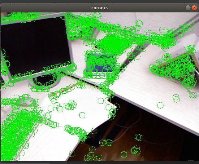
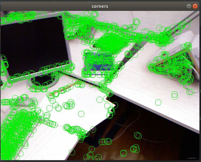
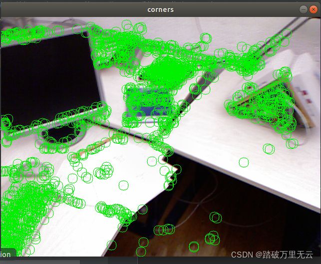
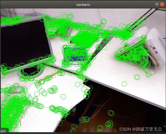
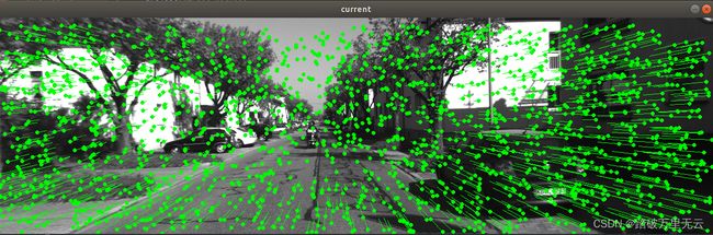
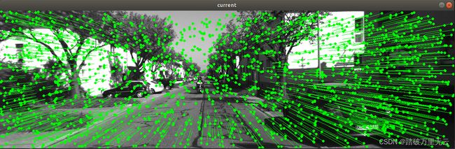
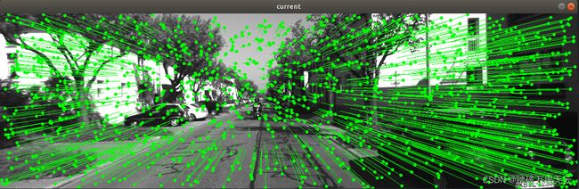
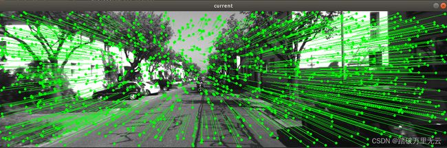
• 我们会用一些实例图片测试直接法的结果，计算相机的位姿
• 为了展示直接法对特征点的不敏感性，随机地在第一张图片中选取一些点，不使用任何角点或特征点提取算法，来看看结果
  
  
  
  
  

3.5 感悟

• 书上p230详细介绍了直接法的优缺点
• 上述的结果图中：每个小圆点是此时的点，而每个点都有一个自己的”尾巴“，这个尾巴的末尾就是该点在之前时刻的位置，所以可以看出，摄像头是向前前进的，从而有一种像素扑面而来的可视化