神经网络 目标跟踪
Multiple object tracking(MOT) is the task of studying object appearance and movements to analyze their trajectories. For a given input video the algorithm is supposed to output which portions of the image represent the same object in different frames of the video. Algorithms like these can be used to solve some exciting problems like analyzing a particular soccer player’s movements during the game, predicting whether a person is going to cross the street or not, or to track and analyze the movement of microscopic organisms in time-lapse microscopy images, etc.
多目标跟踪(MOT)是研究对象外观和运动以分析其轨迹的任务。 对于给定的输入视频,算法应该输出图像的哪些部分代表视频不同帧中的同一对象。 诸如此类的算法可用于解决一些令人兴奋的问题,例如分析特定足球运动员在比赛中的运动,预测某人是否要过马路,或者在延时显微镜中跟踪和分析微观生物的运动。图片等

Multiple object tracking solutions fall into two categories:
多对象跟踪解决方案分为两类:
Online tracking — These algorithms process two frames at a time. They are quite fast which makes them perfect for real-time tracking. These algorithms cannot recover from occlusions or errors. A solution for this is to simply drop the current trajectory and start a new one.
在线跟踪 -这些算法一次处理两个帧。 它们非常快,因此非常适合实时跟踪。 这些算法无法从遮挡或错误中恢复。 一种解决方案是简单地放弃当前轨迹并开始新的轨迹。
Offline tracking — Processes a batch of frames. Since a batch of frames is fed as input to these algorithms they can recover from occlusions or errors. This certainly results in significant computational overhead thereby making them not suitable for real-time applications. These are widely used for video analysis applications.
脱机跟踪 —处理一批框架。 由于将一批帧作为这些算法的输入,因此它们可以从遮挡或错误中恢复。 这无疑会导致大量的计算开销,从而使其不适用于实时应用程序。 这些被广泛用于视频分析应用。
In this article, we will go through a state of the art Offline tracking framework for solving the problem of MOT. The approach that we are about to discuss was published in a paper by the researchers at the Dynamic Vision and Learning Group at TUM. Their proposed algorithm achieved SOTA on MOT15, MOT16, and MOT17 challenges.
在本文中,我们将通过一个最新的脱机跟踪框架来解决MOT问题。 我们将要讨论的方法已由TUM的Dynamic Vision and Learning Group的研究人员发表在一篇论文中 。 他们提出的算法在MOT15,MOT16和MOT17挑战中实现了SOTA。
The authors of the paper propose a network flow formulation of MOT to define a fully differentiable framework based on Message Passing Networks(MPN)
本文的作者提出了MOT的网络流公式,以定义基于消息传递网络(MPN)的完全可区分的框架。
Since MPNs are an integral component of this paper I’m gonna take a few minutes to walk you through what MPNs are and what they do. MPNs come under the realm of deep learning on graphs. Most computer vision happens in the image domain where the order of the pixels is important for the representation of an image and this property is exploited by CNNs to extract the most useful information from a patch of the input image. When we move to a different domain like 3D point clouds[figure 2] we cannot employ our favorite CNN based architectures to capture the most important features and relationships in our input 3D data. This is because point clouds are irregular, there is no sense of order, beginning or ending in them.
由于MPN是本文不可或缺的组成部分,因此我将花几分钟时间向您介绍MPN的含义和作用。 MPN属于图的深度学习领域。 大多数计算机视觉都发生在图像域中,其中像素的顺序对于图像的表示很重要,并且CNN会利用此属性从输入图像的补丁中提取最有用的信息。 当我们移至3D点云之类的不同领域时(图2),我们无法采用我们最喜欢的基于CNN的架构来捕获输入3D数据中最重要的特征和关系。 这是因为点云是不规则的,在它们中没有开始或结束的顺序感。

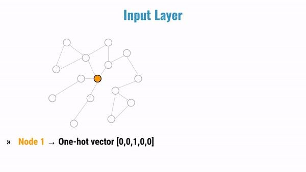
In a typical fully connected network(FCNs) or a CNN, we supply the input in the form of a flattened tensor to the network at the very first layer. In graphical models, we have nodes and edges which are embeddings of the information that we are interested in processing. In FCNs or CNNs we have the concept of layers and our input gets processed layer by layer until it reaches the loss function.
在典型的全连接网络(FCN)或CNN中,我们以展平张量的形式向第一层的网络提供输入。 在图形模型中,我们具有节点和边,它们是我们感兴趣的信息的嵌入。 在FCN或CNN中,我们具有分层的概念,我们的输入会逐层处理,直到达到损失函数为止。
In the case of graphical neural networks(GNNs), there is no concept of a layer so naturally, layer-wise processing of information is absent. Instead, we have an “information propagation” step where a node gets updated by using the info from all neighboring nodes and edges. Once all the nodes in the graph are updated, the processing equivalent of one hidden layer is completed[figure 3]. The graph then goes through a ReLU and the process repeats till the output. If you look at the above figure you will notice that in the second layer the nodes receive information from the nodes that are 2 jumps away. In the third layer, the nodes receive information from nodes that are 3 jumps away, and so on. So, by adding more hidden layers you are receiving information form nodes that are further and further away. Remember that all the information units that are moved are embeddings. The output graph is a graph containing context-aware nodes and edges.
在图形神经网络(GNN)的情况下,没有层的概念,因此自然就没有分层的信息处理方法。 相反,我们有一个“信息传播”步骤,其中节点通过使用来自所有相邻节点和边缘的信息进行更新。 一旦图中的所有节点都更新,相当于一个隐藏层的处理就完成了[图3]。 然后,该图通过ReLU,然后重复该过程,直到输出为止。 如果看上图,您会注意到在第二层中,节点从距离2跳远的节点接收信息。 在第三层中,节点从相距3跳的节点接收信息,依此类推。 因此,通过添加更多隐藏层,您将从越来越远的节点接收信息。 请记住,所有移动的信息单元都是嵌入的。 输出图是包含上下文感知节点和边的图。
Notice that after ‘L’ iterations every node contains information of all the nodes that are at a distance ‘L’ in the graph. This an analogous form of the concept ‘receptive fields’ in CNN, allowing embeddings to capture contextual information. The animation in [figure 4] depicts this well.
注意,在“ L”迭代之后,每个节点都包含图中距离“ L”的所有节点的信息。 这是CNN中“接收域”概念的类似形式,允许嵌入捕获上下文信息。 [图4]中的动画很好地描述了这一点。
Let’s make this a little more concrete with some equations.
让我们通过一些方程使它更加具体。

G — graph with V nodes and E edges, h — embedding, this can be obtained from a CNN or an RNN or any other type of NN. The superscript for ‘h’ is the time step (information propagation step). h(i, j) is the edge embedding between nodes i and j represented as an edge (i,j). h(i) is the node embedding for the node i. The letter “l” represents message-passing steps.
可以从CNN或RNN或任何其他类型的NN获得带有V节点和E边的 G-图 ,h-嵌入 。 “ h”的上标是时间步长(信息传播步长)。 h(i,j)是节点i和j之间的边缘嵌入 ,表示为边缘(i,j) 。 h(i)是为节点i 嵌入的节点。 字母“ l”表示消息传递步骤。
This is the initial organization of the graph[figure 6]. Every node gets features(embeddings) from its neighbors. Yellow box — node embedding, green box — edge embedding
这是图的初始组织[图6]。 每个节点都从其邻居获得特征(嵌入)。 黄色框-节点嵌入,绿色框-边缘嵌入

These embeddings are then combined using some order invariant operation like summation or averaging. The term “message passing” can be inferred from this figure. An order invariant operation is used because of the order-less nature of graphs.[figure 7]
然后使用一些求和不变的运算(例如求和或求平均)来组合这些嵌入。 可以从该图中推断出“消息传递”一词。 由于图的无序性质,因此使用了阶不变操作。[图7]
Below is the equation that represents a message aggregation(“m”) combined with a learnable function [figure 8]. We provide a learnable function to the model so that it can learn which of the nodes are important or relevant and by how much. The order invariant operation here is a summation.
下面的方程式表示结合了可学习函数的消息聚合(“ m”) [图8]。 我们为模型提供了一个可学习的功能,因此它可以了解哪些节点重要或相关,以及多少。 这里的顺序不变运算是求和。
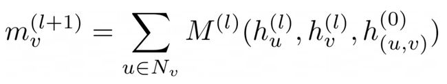
“m” is the message aggregated from the neighbors of “v” to update the node “v”. “u” is a neighbor of “v”. Neighbors of “v” are represented by “Nᵥ”. “M¹” is the learnable function like a NN(neural network)or an MLP(multi-layer perceptron) that takes three inputs — node embedding of neighbor, node embedding of the node to be updated, the embedding of the edge connecting “u” and “v”. All the node update messages follow this equation and the weights of “M¹” are shared across all the nodes.
“ m”是从“ v”的邻居聚合以更新节点“ v”的消息 。 “ u”是“ v”的邻居。 “ v”的邻居用“Nᵥ”表示。 “M¹”是一种可学习的函数,例如NN(神经网络)或MLP(多层感知器) ,它需要三个输入-邻居的节点嵌入,要更新的节点的节点嵌入,连接“ u”的边的嵌入”和“ v” 。 所有节点更新消息均遵循此等式,并且“M¹”的权重在所有节点之间共享 。
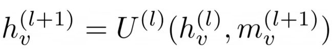
The aggregated message that we just calculated will be used to calculate the new embedding for node “v” at step (l+1)[figure 9]. This completes the update of one node “v”. This is repeated on all the nodes at all information propagation steps. “U¹” is once again a learnable function like NN or MLP which shares weights with all node update operations.
我们刚计算出的聚合消息将用于在步骤(l + 1)中为节点“ v”计算新的嵌入[图9]。 这样就完成了一个节点“ v”的更新。 在所有信息传播步骤的所有节点上重复此操作。 “U¹”再次是可学习的函数,如NN或MLP,它与所有节点更新操作共享权重。
The above two equations [figure 8 and 9] represent a general formulation for a message-passing network. Most message passing networks are an instance of this formulation. Let’s take an example.
以上两个方程式[图8和9]表示消息传递网络的一般公式。 大多数消息传递网络都是这种表达方式的一个实例。 让我们举个例子。
Ex 1:
例1:
MLP₁ is a NN that determines how much of the newly aggregated message is important, MLP₂ determines how important is the embedding of the current node. Note that the learnable function can be MLP or CNN or RNN etc.
MLP 1是一个NN,它确定多少新聚合的消息很重要, MLP 2确定当前节点的嵌入有多重要。 请注意,可学习的功能可以是MLP或CNN或RNN等。
Ex 2: Graph convolutional networks
示例2:图卷积网络

Note that there is a difference in the summation part[figure 10], in this example, we consider a node as a neighbor of itself (self-loop). There is also a change in the normalization term(denominator) of the message aggregation equation to account for this self-loop. “W” is a learnable function.
请注意,求和部分[图10]存在差异,在此示例中,我们将节点视为其自身的邻居(自环) 。 消息聚合方程的归一化项(分母)也发生了变化,以解决此自循环问题。 “ W”是可学习的功能。
The network that we have discussed so far accounts only for node updates. To incorporate edge updates we need to add some more equations. This is done in two steps, Node to Edge update and Edge to Node update. This can be seen in the figure below[figure 11].
到目前为止,我们讨论的网络仅用于节点更新 。 为了合并边缘更新,我们需要添加更多方程。 这分两个步骤完成,即“ 节点到边缘更新”和“ 边缘到节点更新” 。 可以在下图中看到[图11]。
First, we perform “Node to Edge update”, where we generate a new edge embedding. This includes a learnable function “Nₑ” which takes inputs — node embedding for node “i” in the previous step, node embedding for the node “j” in the previous step, and edge embedding for the edge (i,j) from the previous step. Square brackets indicate that these three embeddings are concatenated before feeding to the learnable function[figure 12].
首先,我们执行“节点到边缘更新” ,在此生成新的边缘嵌入。 这包括一个可学习的函数“Nₑ” ,该函数接受输入-上一步中的节点“ i”的节点嵌入,上一步中的节点“ j”的节点嵌入,以及边缘(i,j)的边缘嵌入。前一步。 方括号表示这三个嵌入在馈送给可学习的功能之前是串联的 [图12]。

Next, we perform “Edge to Node update”, where we generate a new node embedding. First, we need to perform an aggregation to generate a message, next we generate the new node embedding by using the computed message aggregation. Here “Φ” is an order invariant operation like mean, sum or max, etc [figure 13].
接下来,我们执行“边缘到节点更新” ,在此生成新的节点嵌入。 首先,我们需要执行聚合以生成一条消息,然后我们使用计算出的消息聚合来生成新的节点嵌入。 此处的“Φ”是阶数不变的运算,例如均值,总和或最大值等[图13]。

This MPN formulation forms the heart of our MOT algorithm. With that brief intro to MPNs lets move on to the main focus of this article, multiple object tracking.
MPN公式构成了我们的MOT算法的核心。 通过对MPN的简短介绍,我们可以继续本文的重点,即多对象跟踪。
The authors of this paper tackle the MOT problem by using the tracking-by-detection paradigm. This two-step approach consists of first generating object detections using any of the popular object detection algorithms like Faster-RCNN, Mask-RCNN, etc. Then use these detections to perform data association using a graphical model. Every node in this graph represents an object detection and an edge between two nodes represents the relationship between the two detections. It is the job of our graphical model to capture higher-order features between two nodes(object detections) by performing message passing. Once the message passing is complete and the edges have converged to their final embeddings a binary classifier is used to perform classification on the edges. Edges belong to two classes, an active edge indicates that the two detections belong to the same trajectory.
本文的作者通过使用“ 检测跟踪”范例解决了MOT问题。 这种分两步的方法包括首先使用任何流行的对象检测算法(例如Faster-RCNN,Mask-RCNN等) 生成对象检测 。然后使用这些检测通过图形模型执行数据关联 。 此图中的每个节点代表一个对象检测 , 两个节点之间的边代表 两个检测之间的 关系 。 通过执行消息传递来捕获两个节点(对象检测)之间的高阶特征是我们图形模型的工作。 一旦消息传递完成并且边缘已经收敛到其最终嵌入,就使用二进制分类 器对边缘进行分类 。 边线属于两类, 活动边线表示这两次检测属于同一轨迹。
A pictorial representation should make things clearer.
图形表示应使情况更清晰。

The above picture [figure 14] shows the output from a detector, frame by frame, starting from time step t, t+1, t+2,… These detections form the nodes of our graph.
上图[图14]从时间步t,t + 1,t + 2等开始逐帧显示检测器的输出。这些检测形成了我们图的节点。
Note that the performance of the proposed algorithm depends on the quality of the detector. All the nodes of the time step “t” are connected to all nodes at time step “t+1”. The job of our graphical model is to find which of these edges belong to the same trajectory.
请注意,所提出算法的性能取决于检测器的质量。 时间步“ t”的所有节点都连接到时间步“ t + 1”的所有节点。 我们的图形模型的工作是找到这些边缘中的哪一条属于同一轨迹。

That’s how our graph would look [figure 16] like after the algorithm has converged. The Red, Yellow, and Green edges represent edges that belong to a particular trajectory and the Blue edges are the ones that do not contribute to a trajectory. The task of dividing a set of detections into trajectories is grouping nodes in the original graph into disconnected components.
这就是算法收敛后的图的样子(图16)。 红色,黄色和绿色边缘代表属于特定轨迹的边缘,蓝色边缘代表对轨迹不起作用的边缘。 将一组检测结果划分为轨迹的任务是将原始图中的节点分组为断开的组件。
Now that the objective of this algorithm is clear let’s pose the problem statement more formally[figure 17]. “O” is the set of input detections, “n” is the total number of objects for all the frames of a video. Every single detection in “O” is represented by small “o”, o = (aᵢ, pᵢ, tᵢ), where aᵢ — raw pixels of the bounding box, pᵢ — 2D image coordinates, tᵢ — timestamp. A trajectory “Tᵢ” is defined as a set of time-ordered object detections that form a trajectory “i”. The goal of MOT is to find a set of these trajectories, T* that can explain the detections present in “O”. Let G = (V, E) be an undirected graph. V — nodes:={1,….n}, and E — edges.
现在,该算法的目标很明确,让我们更正式地提出问题陈述[图17]。 “ O”是输入检测的集合, “ n”是视频所有帧的对象总数。 “ O”中的每个检测都由小“ o”表示 , o =(aᵢ,pᵢ,tᵢ) ,其中aᵢ-边界框的原始像素, pᵢ -2D图像坐标, tᵢ-时间戳。 轨迹“ T 1”被定义为形成轨迹“ i”的一组时间顺序的物体检测 。 MOT的目标是找到这些轨迹的集合T *来解释“ O”中的检测。 令G =(V,E)为无向图 。 V-节点:= {1,.... n},E-边缘。

To perform graph partition we use a binary variable “y ᵢ ⱼ” for every edge between nodes i and j. “y ᵢ ⱼ” is 1 if edge (i, j) belongs to the trajectory Tₖ and Tₖ belongs to T*, 0 otherwise[figure 18].
为了执行图划分,我们对节点i和j之间的每个边使用二进制变量“ yᵢ” 。 如果边(i,j)属于轨迹Tₖ且Tₖ属于T * ,则“ yᵢ ”为1,否则为0 [图18]。
An edge is active when y ᵢ ⱼ = 1. The authors of this paper assume that a node cannot belong to more that one trajectory. So, “y ᵢ ⱼ” has some constraints on it [figure 19].
当y = 1时,边沿有效 。 本文的作者假设一个节点不能属于一个以上的轨迹。 因此,“ yᵢ”对其有一些约束[图19]。

These constraints make sure that every node “i” belongs to V at time step “t” gets linked via an active edge to at most one node in time step t-1 and at most one node in the time step t+1. Every model based on network flows has some sort of constraint that guides the optimization procedure. This is the flow conservation principle used in this approach. A simplified version of the network flow framework is used in this paper. We will not be discussing network flows for MOT in this article but if you are interested I recommend you go through this paper.
这些约束确保了在时间步“ t”处属于V的每个节点“ i”在时间步t-1被经由活动边缘链接到最多一个节点,在时间步t + 1被链接到最多一个节点。 每个基于网络流的模型都具有某种约束,可以指导优化过程。 这就是该方法中使用的流量守恒原理。 本文使用网络流框架的简化版本。 本文不会讨论MOT的网络流,但是如果您有兴趣,我建议您仔细阅读本文 。
Note: I’ve mentioned that the inputs to our graph are detections from the object detector, but this is not the full story. Our detections need to be processed into two particular components — appearance features and motion/geometric features. Our model needs to learn how the objects look like(appearance) and it needs to know the motion or position of the objects so that it can track its trajectory. So, point is that we need to provide appearance information and motion/geometry information to our graphical model. Appearance information is given to the nodes and geometric information is given to the edges.
注意:我已经提到我们图形的输入是来自对象检测器的检测,但这不是全部。 我们的检测需要处理成两个特定的组件- 外观特征和运动/几何特征。 我们的模型需要学习对象的外观(外观),并且需要知道对象的运动或位置,以便可以跟踪其轨迹。 因此,重点是我们需要为图形模型提供外观信息和运动/几何信息。 外观信息提供给节点,几何信息提供给边缘。
Now it’s time to include the content from the MPN section. Given a set of detections the model is supposed to predict the values of the binary variable “y” for every edge of the graph. To achieve this task MPNs are used. There are four stages in the pipeline proposed by the authors of this paper.
现在是时候包括“ MPN”部分中的内容了。 给定一组检测,该模型应该针对图的每个边缘预测二进制变量“ y”的值。 为了实现此任务,使用了MPN。 本文作者提出的流程有四个阶段。
Graph construction — given detections form the nodes of the graph and edges are the connections between the nodes.
图的构造 —给定的检测结果形成了图的节点,并且边缘是节点之间的连接。
Feature encoding — Appearance feature embeddings(node embeddings) are obtained from a CNN applied on the bounding box image. Geometric feature embeddings(edge embeddings) are obtained for a pair of detections in different frames. These are computed by feeding the relative bounding box size, position, and timestamp to an MLP.
特征编码 -外观特征嵌入(节点嵌入)是从应用于边界框图像的CNN获得的。 对于不同帧中的一对检测,获得了几何特征嵌入(边缘嵌入)。 通过将相对边界框的大小,位置和时间戳输入MLP来计算这些值。
Neural message passing — nodes share appearance information and edges share geometric information at each round of message passing. This provides updated embeddings at the end of every round.
神经消息传递 -在每一轮消息传递中 ,节点共享外观信息,边缘共享几何信息。 这样在每个回合结束时提供更新的嵌入。
Training — The edge embeddings generated at the last round of message passing are used to perform binary classification into active and non-active edges. Like all binary classification problems, this model is trained using a cross-entropy loss.
训练 -在消息传递的最后一轮生成的边缘嵌入用于将二进制边缘分类为活动边缘和非活动边缘。 像所有二元分类问题一样,该模型使用交叉熵损失进行训练。
The entire pipeline can be depicted in the following manner [figure 20].
整个管道可以用以下方式描绘[图20]。
At test time we use the model’s predictions per edge(between 0 and 1) and round them off to obtain the final trajectories.
在测试时,我们使用模型的每个边缘的预测(0到1之间)并将其四舍五入以获得最终轨迹。
Remember that the goal of every message passing step is to learn the weights of the learnable functions present in MPN equations so that relevant information gets passed between the nodes and edges. The message passing procedure is the same as that of what we discussed except for a few modifications, let’ talk about those modifications now.
请记住,每个消息传递步骤的目标是学习MPN方程中存在的可学习函数的权重,以便相关信息在节点和边缘之间传递。 消息传递过程与我们讨论的过程相同,只是进行了一些修改,现在让我们谈谈这些修改。
As discussed, this is the equation for a node to edge update.
如所讨论的,这是节点边缘更新的等式。

Edge to node update,
边缘到节点更新 ,
Here ‘Nₑ’ and ‘Nᵥ’ are the learnable functions like MLPs. ‘Nᵢ’ is the set adjacent nodes to the node ‘i’. ‘Φ’ is an order invariant operation like sum, mean, or max [figure 21].
这里的“Nₑ”和“Nᵥ”是可学习的功能,例如MLP。 'Nᵢ'是节点'i'的设置相邻节点。 “Φ”是一阶不变运算,如求和,均值或最大值[图21]。
This what we have seen before now let’s build on top of this. One of the most important contributions of the authors of this paper is introducing Time-Aware Message Passing, a minor but essential tweak to the above equations.
现在,让我们在此基础上进行构建。 本文作者最重要的贡献之一就是介绍了“时间感知消息传递” ,这是对上述方程式的微小但必不可少的调整。
This tweak explicitly encodes the temporal structure of the graph by separating the aggregation step into two parts. The first one is over nodes in the past and the second one is over nodes in the future. The below figure demonstrates how the separation of aggregation is done[figure 22].
通过将聚合步骤分为两部分,此调整可显式编码图的时间结构 。 第一个是过去的节点,第二个是将来的节点。 下图展示了如何完成聚集的分离[图22]。

That’s the whole time aware update. Notice that we are only concerned about changing the equation for edge to node updates. Also notice that now ‘hᵢ⁰’ (initial node embedding) is included in the message computation step.
这是所有时间感知的更新。 注意,我们只关心更改边到节点更新的等式。 还要注意,现在在消息计算步骤中包括了“ h is”(初始节点嵌入) 。
We are towards the end of this article now and there are only two more topics left to discuss. 1) How are these the initial appearance and geometric embeddings generated? 2)How are the training and inference performed?
我们现在到本文的结尾,仅剩下两个主题可以讨论。 1)这些初始外观和几何嵌入是如何生成的? 2)如何进行训练和推理?
- How are these the initial appearance and geometric embeddings generated? 这些初始外观和几何嵌入是如何生成的?
Appearance embeddings — Remember that the global input to this MOT pipeline is the object detections from the detector. These RGB patches of the video frames are fed to a CNN to generate feature embeddings for every detection “oᵢ ∈ O”.
外观嵌入 -请记住,此MOT管道的全局输入是来自检测器的物体检测。 视频帧的这些RGB块被馈送到CNN,以针对每次检测“oᵢ∈O”生成特征嵌入。
That’s how the initial embedding ‘hᵢ⁰’ is calculated. “Nᵥ enc” is the CNN and “aᵢ” is the image patch.
这就是计算初始嵌入“hᵢ⁰”的方式。 “Nᵥenc”是CNN, “aᵢ”是图像块。
Geometric embeddings — These are computed for edges, which means they are computed using a pair of detections in different frames. Here we make use of relative position, size, and distance in time for every pair of detections “oᵢ” and “oⱼ”, tᵢ ≠ tⱼ. We consider the bounding box coordinates, height, and width (xᵢ, yᵢ, hᵢ, wᵢ) and (xⱼ, yⱼ, hⱼ, wⱼ) for calculating relative distance and size.
几何嵌入 -这些是针对边缘计算的,这意味着它们是使用不同帧中的一对检测来计算的。 在这里,我们利用相对位置,大小和时间上的距离来进行每对检测“oᵢ”和“oⱼ”,tᵢ≠tⱼ 。 我们考虑边界框坐标,高度和宽度(xᵢ,yᵢ,hᵢ,wᵢ)和(xⱼ,yⱼ,hⱼ,wⱼ)来计算相对距离和大小。

Once these relative numbers are obtained we concatenate this with the time difference (tᵢ−tⱼ) and the relative appearance. Below the equation for relative appearance [figure 26].
一旦获得这些相对数量我们用的时间差(tᵢ-tⱼ)和相对外观 串联此。 在相对外观方程下面[图26]。
Once we have this concatenated vector with all relative measures in it we feed it to an MLP to obtain the initial edge embedding, “ hᵢ,ⱼ⁰ ”.
一旦有了包含所有相关度量的级联向量,就将其馈送到MLP,以获得初始边缘嵌入“hᵢ,ⱼ⁰” 。
2. How are the training and inference performed?
2.如何进行训练和推理?
An MLP with a sigmoid output is used for the task of edge classification. For every edge (i, j) ∈ E we compute its label by feeding the embeddings of MPN at a given message passing step “l”. Binary cross-entropy loss is used as an objective function.
具有S型输出的MLP用于边缘分类任务 。 对于每个边(i,j)∈E,我们通过在给定的消息传递步骤“ l”中馈入MPN的嵌入来计算其标签。 二元交叉熵损失被用作目标函数。
‘y hat’ — predicted label, ‘y’ — true label.
“ y hat” (预测标签), “ y” (真实标签)。
At inference time we use the edge embeddings of the final message passing step to obtain predictions between 0 and 1 which are rounded off to the nearest integer to get the predicted label values.
在推断时,我们使用最终消息传递步骤的边缘嵌入来获取0到1之间的预测,并四舍五入到最接近的整数以获取预测的标签值。
论文结果 (Paper results)
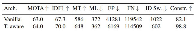
This table shows how time aware message passing update improves tracking performance w.r.t vanilla MPN [figure 28]. (Upward arrow for a score indicates higher the better, a lower arrow indicates lower the better)
下表显示了具有时间意识的消息传递更新如何提高原始MPN的跟踪性能[图28]。 (分数的向上箭头表示越高越好,向下箭头表示越低越好)
Remember that elaborate formulation that we discussed for getting the edge embeddings (concatenation of time difference, relative appearance and, relative position), turns out that this is the best form of embedding for the MOT task [figure 29].
记住,我们为获取边缘嵌入而讨论的精心设计(时差,相对外观和相对位置的串联)证明,这是用于MOT任务的最佳嵌入形式[图29]。
Based on what we have discussed, what’s your take on the relationship between the MOTA score and the number of message passing steps? The higher the message passing steps more contextual information gets captured hence higher MOTA values, right?
根据我们的讨论,您对MOTA分数与邮件传递步骤数之间的关系有何看法? 消息传递步骤越高,捕获到的上下文信息越多,因此MOTA值也就越高,对吗?
Well, that’s not entirely true. MOTA score saturates after a certain point. MOTA score saturates after just 4 message-passing steps! [figure 30]
好吧,这并非完全正确。 MOTA分数在特定点后达到饱和。 仅通过4条消息传递步骤,MOTA分数就会达到饱和! [图30]
Comparing with previous MOT algorithms[figure 31].
与以前的MOT算法相比[图31]。

Phew! That was a pretty long article. If you are with me till here then I’m gonna assume that you are willing to go a little further, so I highly recommend you read the implementation details given in the paper. Thanks for reading :)
! 那是一篇很长的文章。 如果您与我在一起直到现在,那么我将假设您愿意走得更远,因此,我强烈建议您阅读本文中给出的实现细节。 谢谢阅读 :)
参考和推荐阅读 (References and recommended reading)
Original paper
原始纸
MPN and graphical models
MPN和图形模型
Network flows paper
网络流程文件
Everybody needs somebody: Modeling social and grouping behavior on a linear programming multiple people tracker
每个人都需要一个人 :在线性编程多人跟踪器上建模社交和分组行为
CV3DST course at TUM
TUM的CV3DST课程
Neural message passing for quantum chemistry
神经信息传递给量子化学
Semi-supervised classification with graph convolutional networks
图卷积网络的半监督分类
Relational inductive biases, deep learning, and graph networks
关系归纳偏差,深度学习和图网络
翻译自: https://medium.com/@rishikeshdhayarkar1091/graph-neural-networks-for-multiple-object-tracking-ec32f280a945
神经网络 目标跟踪