VGG网络学习笔记。
VGG网络学习
看b站 霹雳吧啦Wz 的视频总结的学习笔记!
视频的地址
大佬的Github代码
1、VGG网络详解
VGG 在2014年由牛津大学著名研究组 VGG(Visual Geometry Group)提出,斩获该年 ImageNet 竞赛中 Localization Task(定位任务)第一名和 Classification Task(分类任务)第二名。
论文:Very Deep Convolutional Networks for Large-Scale Image Recognition
网络中的亮点:通过堆叠多个3*3的卷机核来替代大尺度卷积核(减少训练参数)。
论文中提到,可以通过堆叠两个3×3的卷积核替代5x5的卷积核,堆叠三个3×3的卷积核替代7x7的卷积核,因为他们拥有相同的感受野。
1.1、CNN感受野
先介绍一下什么叫做感受野:
在卷积神经网络中,决定某一层输出结果中一个元素所对应的输入层的区域大小,被称作感受野(receptive field)。通俗的解释是,输出 feature map 上的一个单元对应输入层上的区域大小。
下面举个例子介绍一下,第三层中的一个单元对应第二层中大小为 2*2 的区域,对应第一层中的大小为 5*5 区域。

图中公式中,out 是输出的大小,in 是输入的大小,F 是卷积核的大小,P 为 padding 的大小,S 为步长的大小。
接下来我们看一下感受野的计算公式:

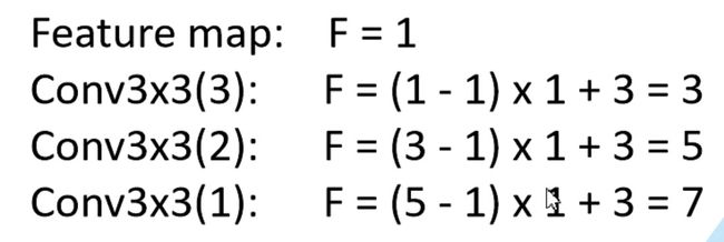
我们刚刚说到,通过堆叠三个 3*3 的卷积核可以替代 7*7 的卷积核,接下来我们通过感受野的计算公式计算一下:
一个特征矩阵通过三个 3*3 的卷积得到 feature map 为1,Stride 默认为1。我们通过公式计算得到最后的 F 为7,因此我们可以证明三个 3*3 的卷积核可以替代一个 7*7 的卷积核。
我们再计算一下堆叠三个 3*3 的卷积核后的训练参数是不是减少了。
训练参数总数 = 卷积核的大小 * 输入的C * 输出的C(卷积核的组数) * 堆叠卷积核的个数

因此,我们可以看出使用的训练参数减少了。
1.2、VGG16详解

VGG 网络有很多版本,如图中表所示,我们一般常用 D ,也就是 vgg16 模型。
接下来我们详细介绍一下 vgg16 计算的过程:
- 首先,输入一张
224*224*3的 RGB 图像。 - 然后,经过两层卷积层,并 ReLU 激活,卷积核大小为
3*3,卷积核的组数为64(也就是输出的大小),得到的维度为224*224*64。 - 然后,经过 maxpooling 最大池化层,得到的维度为
112*112*64。 - 然后,再经过两层卷积层,卷积核的组数为128,得到的维度为
112*112*128。 - 然后,经过 maxpooling 最大池化层,得到的维度为
56*56*128。 - 然后,再经过三层卷积层,卷积核的组数为256,得到的维度为
56*56*256。 - 然后,经过 maxpooling 最大池化层,得到的维度为
28*28*256。 - 然后,再经过三层卷积层,卷积核的组数为512,得到的维度为
28*28*512。 - 然后,经过 maxpooling 最大池化层,得到的维度为
14*14*512。 - 然后,再经过三层卷积层,卷积核的组数为512,得到的维度为
14*14*512。 - 然后,经过 maxpooling 最大池化层,得到的维度为
7*7*512。 - 然后,经过三层的全连接层并做 ReLU 激活(最后一层不做ReLU激活,因为要做softmax),三层的节点分别为4096、4096、1000。
- 最后,经过 softmax 得到输出结果。
2、使用pytorch搭建VGG网络
2.1、model
VGG模型可以分为提取特征网络结构和分类网络结构两个部分。
提取特征网络结构是前面的卷积层和最大池化层;分类网络结构是后面的全联接层和softmax层。
import torch.nn as nn
import torch

# official pretrain weights
model_urls = {
    'vgg11': 'https://download.pytorch.org/models/vgg11-bbd30ac9.pth',
    'vgg13': 'https://download.pytorch.org/models/vgg13-c768596a.pth',
    'vgg16': 'https://download.pytorch.org/models/vgg16-397923af.pth',
    'vgg19': 'https://download.pytorch.org/models/vgg19-dcbb9e9d.pth'
}


class VGG(nn.Module):
    def __init__(self, features, num_classes=1000, init_weights=False):
        super(VGG, self).__init__()
        self.features = features
        # 分类网络结构:三个全联接层。
        self.classifier = nn.Sequential(
            nn.Linear(512*7*7, 4096),
            nn.ReLU(True),
            nn.Dropout(p=0.5), # 以50%的概率随即失活神经元,目的为了方式过拟合
            nn.Linear(4096, 4096),
            nn.ReLU(True),
            nn.Dropout(p=0.5),
            nn.Linear(4096, num_classes) # num_classes为分类的类别数
        )
        if init_weights: # 是否初始化权重参数
            self._initialize_weights()

    def forward(self, x):
        # N x 3 x 224 x 224
        x = self.features(x) # 提取特征网络结构
        # N x 512 x 7 x 7
        x = torch.flatten(x, start_dim=1) # 沿着通道维度进行展平处理
        # N x 512*7*7
        x = self.classifier(x) # 分类网络结构
        return x

    def _initialize_weights(self):
        for m in self.modules(): # 遍历模型中的每一层
            if isinstance(m, nn.Conv2d): # 如果该层为卷积层
                # nn.init.kaiming_normal_(m.weight, mode='fan_out', nonlinearity='relu')
                nn.init.xavier_uniform_(m.weight) # 初始化权重参数
                if m.bias is not None: # 如果偏置存在的话,初始化为0
                    nn.init.constant_(m.bias, 0)
            elif isinstance(m, nn.Linear): # 如果为线性层
                nn.init.xavier_uniform_(m.weight)
                # nn.init.normal_(m.weight, 0, 0.01)
                nn.init.constant_(m.bias, 0)


# 提取特征网络结构。
def make_features(cfg: list):
    layers = [] # 存放每一层定义的结构
    in_channels = 3 # RGB图片,输入的通道为3
    for v in cfg:
        if v == "M":
            layers += [nn.MaxPool2d(kernel_size=2, stride=2)]
        else:
            conv2d = nn.Conv2d(in_channels, v, kernel_size=3, padding=1)
            layers += [conv2d, nn.ReLU(True)]
            in_channels = v # 下次层的输入通道数为这一层的输出通道数
    return nn.Sequential(*layers) # * 代表通过为关键字参数的形式输入


# 字典配置:key值为对应版本的vgg模型;value值中数字为输出通道大小(卷积核组数),M为最大池化层。
cfgs = {
    'vgg11': [64, 'M', 128, 'M', 256, 256, 'M', 512, 512, 'M', 512, 512, 'M'],
    'vgg13': [64, 64, 'M', 128, 128, 'M', 256, 256, 'M', 512, 512, 'M', 512, 512, 'M'],
    'vgg16': [64, 64, 'M', 128, 128, 'M', 256, 256, 256, 'M', 512, 512, 512, 'M', 512, 512, 512, 'M'],
    'vgg19': [64, 64, 'M', 128, 128, 'M', 256, 256, 256, 256, 'M', 512, 512, 512, 512, 'M', 512, 512, 512, 512, 'M'],
}


# 初始化模型。
def vgg(model_name="vgg16", **kwargs): # ** 代表输入的参数为可变长度的字典变量,参数可以是多个。
    assert model_name in cfgs, "Warning: model number {} not in cfgs dict!".format(model_name)
    cfg = cfgs[model_name] # 通过key值(模型的名字)得到value值。

    model = VGG(make_features(cfg), **kwargs)
    return model
2.2、train
import os
import sys
import json

import torch
import torch.nn as nn
from torchvision import transforms, datasets
import torch.optim as optim
from tqdm import tqdm

from model import vgg


def main():
    # 是否使用GPU。
    device = torch.device("cuda:0" if torch.cuda.is_available() else "cpu")
    print("using {} device.".format(device))

    # 数据预处理。
    data_transform = {
        "train": transforms.Compose([transforms.RandomResizedCrop(224), # 随机裁剪
                                     transforms.RandomHorizontalFlip(), # 随机水平翻转
                                     transforms.ToTensor(),
                                     # 标准化处理:三个维度,均值和方差都为0.5,(x-均值)/方差
                                     transforms.Normalize((0.5, 0.5, 0.5), (0.5, 0.5, 0.5))]),
        "val": transforms.Compose([transforms.Resize((224, 224)),
                                   transforms.ToTensor(),
                                   transforms.Normalize((0.5, 0.5, 0.5), (0.5, 0.5, 0.5))])}

    # 获取根目录, ../.. 代表返回上上级目录。getcwd是得到当前项目路径,join是拼接路径。
    data_root = os.path.abspath(os.path.join(os.getcwd(), "../.."))  # get data root path
    # 拼接数据集的路径。
    image_path = os.path.join(data_root, "data_set", "flower_data")  # flower data set path
    assert os.path.exists(image_path), "{} path does not exist.".format(image_path)
    # 训练数据集。
    train_dataset = datasets.ImageFolder(root=os.path.join(image_path, "train"),
                                         transform=data_transform["train"])
    train_num = len(train_dataset) # 返回训练数据集的图片个数。

    # {'daisy':0, 'dandelion':1, 'roses':2, 'sunflower':3, 'tulips':4}
    flower_list = train_dataset.class_to_idx   # 返回数据集类别对应的索引
    cla_dict = dict((val, key) for key, val in flower_list.items()) # 把key和value颠倒过来
    # write dict into json file
    # 编码成json文件,并保存。
    json_str = json.dumps(cla_dict, indent=4)
    with open('class_indices.json', 'w') as json_file:
        json_file.write(json_str)

    batch_size = 32
    # 线程的个数,windows只能设置为0,表示使用主线程。
    nw = min([os.cpu_count(), batch_size if batch_size > 1 else 0, 8])  # number of workers
    print('Using {} dataloader workers every process'.format(nw))

    # 加载训练数据集。
    train_loader = torch.utils.data.DataLoader(train_dataset,
                                               batch_size=batch_size, shuffle=True,
                                               num_workers=nw)

    # 验证数据集。
    validate_dataset = datasets.ImageFolder(root=os.path.join(image_path, "val"),
                                            transform=data_transform["val"])
    val_num = len(validate_dataset)   # 返回验证数据集的图片个数
    # 加载验证数据集。
    validate_loader = torch.utils.data.DataLoader(validate_dataset,
                                                  batch_size=batch_size, shuffle=False,
                                                  num_workers=nw)
    print("using {} images for training, {} images for validation.".format(train_num,
                                                                           val_num))

    # test_data_iter = iter(validate_loader)
    # test_image, test_label = test_data_iter.next()

    model_name = "vgg16"
    net = vgg(model_name=model_name, num_classes=5, init_weights=True) # 初始化模型
    net.to(device)
    loss_function = nn.CrossEntropyLoss()
    optimizer = optim.Adam(net.parameters(), lr=0.0001)

    epochs = 30
    best_acc = 0.0 # 最优准确率
    save_path = './{}Net.pth'.format(model_name) # 保存模型的路径
    train_steps = len(train_loader)
    for epoch in range(epochs):
        # train
        net.train() # 在训练时使用dropout
        running_loss = 0.0
        train_bar = tqdm(train_loader, file=sys.stdout) # 进度条
        for step, data in enumerate(train_bar):
            images, labels = data
            optimizer.zero_grad()
            outputs = net(images.to(device))
            loss = loss_function(outputs, labels.to(device))
            loss.backward()
            optimizer.step()

            # print statistics
            running_loss += loss.item()

            # 打印进度条。
            train_bar.desc = "train epoch[{}/{}] loss:{:.3f}".format(epoch + 1,
                                                                     epochs,
                                                                     loss)

        # validate
        net.eval() # 在验证时不使用dropout
        acc = 0.0  # accumulate accurate number / epoch
        with torch.no_grad(): # 不计算梯度
            val_bar = tqdm(validate_loader, file=sys.stdout)
            for val_data in val_bar:
                val_images, val_labels = val_data
                outputs = net(val_images.to(device))
                # 预测最大可能的类别,dim=1表示类别,[1]表示返回索引即可。
                predict_y = torch.max(outputs, dim=1)[1]
                acc += torch.eq(predict_y, val_labels.to(device)).sum().item()

        val_accurate = acc / val_num # 计算平均准确率
        # 打印验证信息。
        print('[epoch %d] train_loss: %.3f  val_accuracy: %.3f' %
              (epoch + 1, running_loss / train_steps, val_accurate))

        # 得到最优的准确率,并保存模型的权重。
        if val_accurate > best_acc:
            best_acc = val_accurate
            torch.save(net.state_dict(), save_path)

    print('Finished Training')


if __name__ == '__main__':
    main()
2.3、predict
import os
import json

import torch
from PIL import Image
from torchvision import transforms
import matplotlib.pyplot as plt

from model import vgg


def main():
    device = torch.device("cuda:0" if torch.cuda.is_available() else "cpu")

    # 数据预处理。
    data_transform = transforms.Compose(
        [transforms.Resize((224, 224)),
         transforms.ToTensor(),
         transforms.Normalize((0.5, 0.5, 0.5), (0.5, 0.5, 0.5))])

    # load image
    img_path = "./tulip.jpg"
    assert os.path.exists(img_path), "file: '{}' dose not exist.".format(img_path)
    img = Image.open(img_path) # 加载图片
    plt.imshow(img) # 展示图片
    # [N, C, H, W]
    img = data_transform(img) # 预处理图片
    # expand batch dimension
    img = torch.unsqueeze(img, dim=0) # 加一个batch维度

    # read class_indict
    json_path = './class_indices.json'
    assert os.path.exists(json_path), "file: '{}' dose not exist.".format(json_path)

    # 解码json文件。
    with open(json_path, "r") as f:
        class_indict = json.load(f)

    # create model
    model = vgg(model_name="vgg16", num_classes=5).to(device) # 初始化模型
    # load model weights
    weights_path = "./vgg16Net.pth"
    assert os.path.exists(weights_path), "file: '{}' dose not exist.".format(weights_path)
    model.load_state_dict(torch.load(weights_path, map_location=device)) # 加载模型的权重

    model.eval() # 在验证时不使用dropout
    with torch.no_grad():
        # predict class
        output = torch.squeeze(model(img.to(device))).cpu()
        predict = torch.softmax(output, dim=0)
        predict_cla = torch.argmax(predict).numpy() # 得到概率最大的类别的下标

    # 打印信息。
    print_res = "class: {}   prob: {:.3}".format(class_indict[str(predict_cla)],
                                                 predict[predict_cla].numpy())
    plt.title(print_res)
    # 遍历每个类别的概率。
    for i in range(len(predict)):
        print("class: {:10}   prob: {:.3}".format(class_indict[str(i)],
                                                  predict[i].numpy()))
    plt.show()


if __name__ == '__main__':
    main()
2.4、运行项目
我的电脑性能不高,运行不了!
首先,我们需要下载数据集,在大佬的 github 下载,里面有详细的下载步骤。
数据集下载地址
然后,运行 train.py 文件,会生成一个json文件,并得到一个训练好的模型。
{
    "0": "daisy",
    "1": "dandelion",
    "2": "roses",
    "3": "sunflowers",
    "4": "tulips"
}
然后,我们需要把需要预测的图片放在对应的路径,运行 predict.py 文件,查看结果!