随机森林多重插补数据_python中带有随机森林的多重插补

随机森林多重插补数据

Missing data is a common problem in data science — one that tends to cause a lot of headaches. Some algorithms simply can’t handle it. Linear regression, support vector machines, and neural networks are all examples of algorithms which require hacky work-arounds to make missing values digestible. Other algorithms, like gradient boosting (lightGBM and xgboost specifically), have elegant solutions for missing values. However, that doesn’t mean they can’t still cause problems.

数据丢失是数据科学中的常见问题-往往会引起很多麻烦。 有些算法根本无法处理。 线性回归，支持向量机和神经网络都是算法的示例，这些算法需要巧妙的解决方法才能使缺失值易于消化。 其他算法，例如渐变增强(特别是lightGBM和xgboost)，对于缺失值也有很好的解决方案。 但是，这并不意味着它们仍然不会引起问题。

There are several situations when missing data can result in bias predictions, even in models that have native handling of missing values:

在某些情况下，即使在具有本机处理缺失值的模型中，缺失数据也会导致偏差预测：

• Missing data is overwritten, and is only sometimes available at time of inference. This is especially common in funnel modeling, where more becomes known about the customer as they make it further in the funnel.
  丢失的数据将被覆盖，并且有时仅在推断时可用。 这在渠道建模中尤为常见，因为随着客户在渠道中的不断发展，对客户的了解越来越多。
• The mechanism that causes missing data changes — examples would be new questions on a website, new vendor, etc. This is especially a problem if the mechanism is related to the target you ultimately want to model.
  导致丢失数据更改的机制-例如网站，新供应商等上的新问题。如果该机制与您最终要建模的目标有关，则尤其是一个问题。

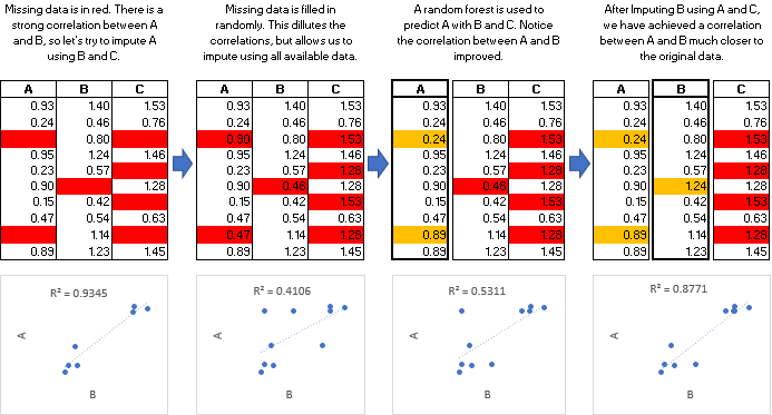
If only we could know what those missing values actually were, and use them. Well, we can’t. But we can do the next best thing: Estimate their values with Multiple Imputation by Chained Equations (MICE):

如果我们只能知道那些缺失值实际上是什么，并使用它们。 好吧，我们不能。 但是我们可以做下最好的事情：通过链式方程(MICE)的多重插补估算其值：

miceforest Github miceforest Github

MICE算法 (The MICE Algorithm)

Multiple Imputation by Chained Equations, also called “fully conditional specification”, is defined as such:

链式方程的多重插补，也称为“完全条件规范”，其定义如下：

Uploaded by Author 由作者上传

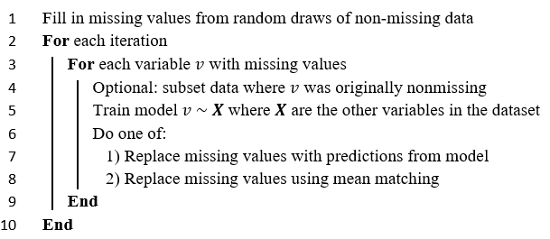
This process is repeated for the desired number of datasets. The method mentioned on line 8, mean matching, is used to produce imputations that behave more like the original data. This idea is explored in depth in Stef van Buuren’s online book. A reproducible example of the effects on mean matching can also be found on the miceforest Github page.

对所需数量的数据集重复此过程。 第8行提到的方法，均值匹配，用于产生行为，其行为更像原始数据。 Stef van Buuren的在线书对此概念进行了深入探讨。 关于均值匹配的影响的可重现示例也可以在miceforest Github页面上找到。

Multiple iterations are sometimes required for the imputations to converge. There are several things that affect how many iterations are required to achieve convergence such as the type of missing data, the information density in the dataset, and the model used to impute the data.

有时需要多次迭代才能使插补收敛。 有几件事会影响实现收敛所需的迭代次数，例如丢失数据的类型，数据集中的信息密度以及用于估算数据的模型。

Technically, any predictive model capable of inference can be used for MICE. In this article, we impute a dataset with the miceforest Python library, which uses random forests. Random forests work well with the MICE algorithm for several reasons:

从技术上讲，任何能够推理的预测模型都可以用于MICE。 在本文中，我们使用miceforest Python库估算了数据集，该库使用随机森林。 出于以下几个原因，随机森林可与MICE算法配合使用：

1. Do not need much hyperparameter tuning
   不需要太多的超参数调整
2. Easily handle non-linear relationships in the data
   轻松处理数据中的非线性关系
3. Can return OOB performance inexpensively
   可以廉价地返回OOB性能
4. Are trivially parallelizable
   几乎可以并行化
5. Can return feature importance for diagnostics
   可以返回功能重要性以进行诊断

一个实际的例子(A Practical Example)

Let’s load our packages and data. We use the iris dataset, imported from sklearn:

让我们加载我们的包和数据。 我们使用从sklearn导入的虹膜数据集：

import miceforest as mf
from sklearn.datasets import load_iris
import pandas as pd

# Load and format data
iris = pd.concat(load_iris(as_frame=True,return_X_y=True),axis=1)
iris.rename(columns = {'target':'species'}, inplace = True)
iris['species'] = iris['species'].astype('category')

# Introduce missing values
iris_amp = mf.ampute_data(iris,perc=0.25,random_state=1991)

We simply need to create a MultipleImputedKernel and perform mice for a few iterations:

我们只需要创建一个MultipleImputedKernel并执行鼠标几次迭代即可：

# Create kernels. 
kernel = mf.MultipleImputedKernel(
  data=iris_amp,
  save_all_iterations=True,
  random_state=1991
)

# Run the MICE algorithm for 3 iterations on each of the datasets
kernel.mice(3,verbose=True)

What we have done is created 5 separate datasets with different imputed values. We can never be sure what the original data was, but if our different datasets all come up with similar imputed values, we can say that we are confident in our imputations. Let’s take a look at the correlations of the imputed values between datasets:

我们所做的是创建5个具有不同估算值的独立数据集。 我们永远无法确定原始数据是什么，但是如果我们不同的数据集都具有相似的估算值，则可以说我们对估算有信心。 让我们看一下数据集之间的估算值的相关性：

kernel.plot_correlations(wspace=0.4,hspace=0.5)

Uploaded by Author 由作者上传

Each dot represents the correlation of imputed values between 2 of the datasets. Every combination of datasets is included in the graph. If the correlation between imputed values is low, it means we did not impute the values with much confidence. It looks like our models all pretty much agreed on the imputations for petal length and petal width. If we ran more iterations, we might be able to get better results for sepal length and sepal width as well.

每个点表示两个数据集之间的估算值的相关性。 图中包括数据集的每个组合。 如果估算值之间的相关性很低，则意味着我们没有很自信地估算值。 看起来我们的模型在花瓣长度和花瓣宽度的估算上几乎完全一致。 如果我们运行更多的迭代，则对于隔片长度和隔片宽度，我们也可能会获得更好的结果。

估算新数据 (Imputing New Data)

Multiple imputation by chained random forests can take a long time, especially if the dataset is we are imputing is large. What if we want to use this method in production? It turns out we can save the models we fit during the original MICE procedure, and use them to impute a new dataset:

链式随机森林的多次插补可能会花费很长时间，尤其是如果我们要插补的数据集很大。 如果我们想在生产中使用这种方法怎么办？ 事实证明，我们可以保存在原始MICE过程中适合的模型，并使用它们来估算新的数据集：

# Our new dataset
new_data = iris_amp.iloc[range(50)]# Make a multiple imputed dataset with our new data
new_data_imputed = kernel.impute_new_data(new_data)# Return a completed dataset
new_completed_data = new_data_imputed.complete_data(0)

miceforest re-creates the process of the original procedure on the new data without updating the models at each iteration. This saves a significant amount of time. We can also query this new dataset to see if the correlations have converged, or even plot the distributions of the imputations:

miceforest在新数据上重新创建原始过程的过程，而无需在每次迭代时更新模型。 这样可以节省大量时间。 我们还可以查询这个新的数据集，以查看相关性是否已经收敛，甚至可以绘制插补的分布图：

new_data_imputed.plot_imputed_distributions(wspace=0.35,hspace=0.4)

Uploaded by Author 由作者上传

建立置信区间(Building Confidence Intervals)

Now that we have our 5 datasets, you may be tempted to take the average imputed value to create a single, final dataset, and be done with it. If you are performing a traditional statistical analysis, this is not recommended — imputations with more variance will tend to revert towards the mean, and the variance of overall imputations will be lowered, resulting in a final dataset which does not behave like the original. It is better to perform multiple analysis and keep track of the variances that are produced by these multiple analysis.

现在我们有了5个数据集，您可能会想求平均值的估算值来创建单个最终数据集，并对其进行处理。 如果您正在执行一个传统的统计分析，不建议这样做-更方差插补将趋向于向均值回复和整体插补的差异将被降低，导致不表现得像原来最后的数据集。 最好执行多重分析并跟踪这些多重分析产生的方差。

Since we have 5 different datasets, we can now train multiple models and build confidence intervals on the results. Here, we train 5 different linear regression models on ‘sepal length (cm)’, and build an assumption about the distribution of the intercept term using the mean and variance of the intercept obtained from our 5 models:

由于我们有5个不同的数据集，我们现在可以训练多个模型并在结果上建立置信区间。 在这里，我们在“间隔长度(cm)”上训练了5个不同的线性回归模型，并使用从我们5个模型中获得的截距的均值和方差建立了关于截距项分布的假设：

from sklearn.linear_model import LinearRegression# For each imputed dataset, train a linear regression
# on 'sepal length (cm)'
intercepts = []
target = 'sepal length (cm)'
for d in range(kernel.dataset_count()):
    comp_dat = kernel.complete_data(d)
    comp_dat = pd.get_dummies(comp_dat)
    X, y = comp_dat.drop(target,1), comp_dat[target]
    model = LinearRegression()
    model.fit(X,y)
    intercepts.append(model.intercept_)# Load packages for plotting
import numpy as np
import matplotlib.pyplot as plt
from scipy.stats import norm

# Make plot.
x_axis = np.arange(1.93, 2.01, 0.0001)
avg_intercept = round(np.mean(intercepts),2)
var_intercept = round(np.var(intercepts),4)
plt.plot(
    x_axis,
    norm.pdf(x_axis,avg_intercept,var_intercept)
)
plt.title(f"""
    Assumed Distribution of Intercept Term
    n=5, mean = {avg_intercept}, variance = {var_intercept}
    """
)

Uploaded by Author 由作者上传

We don’t know what the true intercept term would be if we had no missing values, however we can now make (weak) statements about what the intercept probably would be if we had no missing data. If we wanted to increase n in this scenario, we would need to add more datasets.

我们不知道如果没有缺失值，那么真正的截距项将是什么，但是现在我们可以对没有数据缺失的情况下的截距进行(弱)声明。 如果要在这种情况下增加n，则需要添加更多数据集。

Similar confidence intervals can be run on the coefficients in the linear models, as well as the actual predictions for each sample. Samples with more missing data tend to have wider variance in their predictions in the final model, since there is more chance for the imputed values to differ between datasets.

可以对线性模型中的系数以及每个样本的实际预测运行类似的置信区间。 缺少更多数据的样本在最终模型中的预测中往往具有更大的方差，因为估算值在数据集之间存在差异的可能性更大。

结论 (In conclusion)

We have seen how the MICE algorithm works, and how it can be combined with random forests to accurately impute missing data. We have also gone through a simple example of how multiple imputed datasets can be used to help us build an assumption about how our model parameters are distributed.

我们已经了解了MICE算法的工作原理，以及如何将其与随机森林结合起来以准确估算缺失的数据。 我们还通过了一个简单的示例，说明如何使用多个估算数据集来帮助我们建立关于模型参数如何分布的假设。

翻译自: https://towardsdatascience.com/multiple-imputation-with-random-forests-in-python-dec83c0ac55b

随机森林多重插补数据